Graph neural networks (GNN) represent a powerful class of deep neural network architectures. In an increasingly interconnected world, most information can be modeled as graphs due to the connectivity of information. For example, the atoms in a compound are nodes and the bonds between them are edges.
The beauty of graph neural networks is their ability to operate directly on graph-structured data without sacrificing important details. This is particularly evident when dealing with complex data sets such as chemical compounds, where GNNs allow us to fully exploit the richness of the underlying graphical representation. By doing so, GNNs are able to more fully understand the relationships between atoms and bonds, opening the way to more accurate and in-depth analyses.

Beyond the realm of chemistry, the impact of graph structures extends to different fields. Take transportation data as an example, where cities are nodes and the routes between them are edges. GNNs have proven invaluable in tasks such as traffic jam prediction, proving their effectiveness in capturing the complex dynamics of urban mobility. The ability of GNNs to grasp the spatial dependencies and patterns inherent in graph data becomes a powerful tool when faced with challenges such as predicting traffic congestion. Numerous models based on GNN have emerged as state-of-the-art solutions for predicting traffic congestion, becoming the most cutting-edge models. The following is a model for predicting traffic jams on paperswithcode. Basically, it is all GNN.  This article will introduce the theoretical basis of graph convolution. By delving into the complexity of the graph Fourier transform and its connection to graph convolution, we will lay the foundation for a deeper understanding of this key concept in the world of GNNs.
How to define graph convolution
The core concept of GNN lies in graph convolution, which achieves effective processing of graph data by capturing the relationship between nodes and edges. Among the various methods for understanding graph convolution, this article focuses on using the theory of graph Fourier transform to explain it. This concept provides a unique perspective into the mechanics of graph convolution. The graph Fourier transform allows us to represent graph signals - data associated with nodes - in terms of graph frequencies. This decomposition, based on spectral analysis, provides insights into underlying patterns and structures in the graph. Some GNN architectures utilize attention mechanisms and other advanced methods that go beyond graph convolution. However, we mainly discuss the nature of graph convolution and its interaction with graph Fourier transform, so parts such as attention are not within the scope of this article.
What is the graph Fourier transform?
The concept of graph Fourier transform has interesting similarities with the classical Fourier transform. Just like the traditional Fourier transform decomposes a wave signal into its component frequencies, the graph Fourier transform operates on graph-structured data, revealing the frequencies of the signal embedded within it. Imagine a weighted undirected graph without cycles or multiple edge structures. The graph Fourier transform is a mathematical operation that emphasizes the transformation of the signal present on the graph. This concept becomes particularly illustrative in the case of signal dimensionality equal to 1. Consider the following description, which depicts what a signal looks like on a chart [1]. 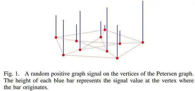 Decomposing a signal into a graph of frequencies, or the graph Fourier transform, provides a way to identify the various relationships, patterns, and complexities inherent in graphical data.
graph Laplacian
To understand the Fourier transform of a graph, we will begin a basic exploration by first introducing the Laplace transform of a graph. This key concept is the cornerstone of revealing the natural frequency characteristics of graphics. The graph Laplacian is denoted L and is defined as:  In this equation, A represents the adjacency matrix, which encodes the connections between nodes in the graph, and D represents the degree matrix, which captures the degree of each node. Since D and A are real symmetric matrices, the graph Laplacian matrix also has the properties of a real symmetric matrix. This property allows us to perform spectral decomposition of the graph Laplacian function, expressed as:
 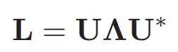 In the above formula, U represents the eigenvector matrix, Λ is the diagonal composed of eigenvalues (Λ 1, Λ 2,..., Λ n) matrix.
Quadratic
This section explains what the quadratic and quadratic forms of a Laplacian graph mean, and how it relates to the frequency of the graph signal. The quadratic form of graph Laplacian can be defined as: 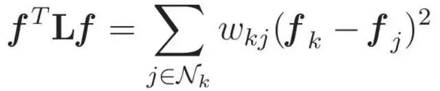 where f represents the graph signal, w represents the weight of an edge, and Nk represents the set of nodes connected to node k. This representation reveals two fundamental key aspects: Smoothness of the function The quadratic form provides insight into the smoothness of the function on the graph. Consider the scenario of f =[1,1,1,…,1]T. According to the definition of the graph Laplacian, the quadratic form evaluates to zero. That is, the smoother the function is across nodes, the smaller the resulting quadratic form will be. This interaction provides a mechanism to quantify the inherent smoothness of a graphical signal. The quadratic form of similarity between adjacent nodes is also used as a measure to evaluate the similarity between signals on adjacent nodes. When the difference between f(i) and f(j) is large, the corresponding quadratic value increases proportionally. Conversely, if the signals at adjacent nodes are similar, the quadratic form approaches zero. This observation is consistent with the idea that larger values of the quadratic form reflect greater variation between adjacent nodes. With these concepts in mind, quadratic forms can be interpreted as surrogates for the "frequency" of a function on a graph. By utilizing the information it provides, we can perform graphical signal decomposition based on frequency components. This critical step is a precursor to the graph Fourier transform, unlocking a powerful method to reveal frequency features embedded in graph-structured data.
Graph Fourier Transform
We have established the quadratic shape of the Laplacian plot as an indicator of signal frequency, where larger quadratic values represent higher frequencies. One more important point: be aware that these values may be affected by the norm of f. To ensure consistency and eliminate the potential impact of different norms, we also need to impose the constraint that the norm of f equals 1. In order to obtain the stationary value of the quadratic form under norm conditions, we utilize the powerful optimization technique of the Lagrange multiplier method. Applying appropriate transformations to this problem, we end up with an eigenvalue problem: 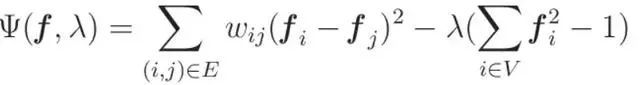
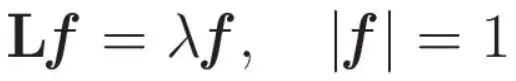 This eigenvalue provides a relation: each eigenvalue of L reflects the value of the quadratic form of the graph Laplacian. Simply put, these eigenvalues capture the frequency at which the pattern signal vibrates. In this way we have a basic understanding of eigenvalues as indicators of function frequency. The connection between eigenvectors and graph Laplacians becomes the means to perform a graph Fourier transform—a process that systematically reveals the intrinsic frequency elements of a graph signal. Now, we can look at the definition of Fourier transform
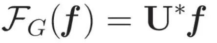
From graph Fourier transform to graph convolution
With the graph Fourier transform introduced above, we have obtained a powerful tool for effectively analyzing and processing graph signals. In our study we study the connection between graph Fourier transform and graph convolution. The core of this connection is the convolution theorem, which establishes the connection between the convolution operation and the product of elements in the Fourier domain. 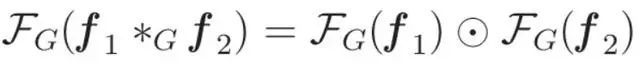 The convolution operation is similar to the element-wise multiplication of the transformed signal in the Fourier domain. An indirect definition of graph convolution can be derived using the convolution theorem:
- Perform Fourier transform on the graphic signal.
- Multiply the transformed signal with a learnable weight vector.
- Perform the inverse Fourier transform on the element-wise product to obtain the output of the graph convolution.
The formula for graph convolution can now be stated as follows: 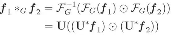 To make this definition more streamlined, we introduce a practical parameterization. Since the element-wise product with U*f can be expressed as the product with diag(U*f), s, let the learnable weight θ be: By taking advantage of
 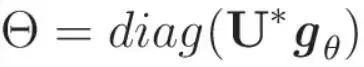 this parameterization, the graph convolution formula of gθ adopts a simplified sum Intuitive form:
 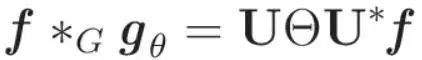 Look, we have defined a graph convolution from the Fourier transform of the graph!
Summarize
In this article, we start by revealing the basic principles of graph Laplacian, and then delve into the basic concept of graph convolution, which is the derivation of graph Fourier transform. The reasoning made in this article should be able to deepen your understanding of the nature of graph convolution.