[Graph Convolution Network] 02-Introduction to Spectral Domain Graph Convolution

Note: This article is a video note on the introduction of spectral domain graph convolution in Chapter 2 , which is only for personal learning use

---

---

1. Introduction to graph convolution

1.1 The Rapid Development of Graph Convolutional Networks

• 16 years ago, there were only 1-2 related documents per year

• In 2018, there were about 7-8 articles in some conferences

• In 19 years, the number of articles has grown explosively, and there are 49 articles in just one conference of NIPS

1.2 Review, the classic convolutional neural network has been successful in many fields

1.3 Two types of data

Regular data (Euclidean space)	Irregular data (non-Euclidean space)
Voice: 1D vector; Image: 2D matrix; Video: 3D matrix	Social data, molecular structure, human skeleton

1.4 Limitations of Classical Convolutional Neural Networks: Cannot Handle Graph Data Structures

Limitations of classical convolution processing graph-structured data:

• Can only handle data with fixed input dimensions
• Local input must be in order

1.5 Extending convolution to graph-structured data

1. Frequency domain: refers to the domain that converts signals into frequencies, and studies the frequency characteristics of signals through frequency analysis. A common transformation method is to use the Fourier transform. In the frequency domain, a signal can be represented as the relative strength of the various frequency components.
2. Spectral domain: refers to the domain that converts signals into energy or power, and studies the energy or power distribution of signals through the analysis of energy or power. A common conversion method is to use the power spectral density function. In the spectral domain, a signal can be expressed as the energy or power of each frequency component.
3. Space domain: refers to the domain that converts signals into spatial coordinates, and studies the spatial characteristics of signals through the analysis of spatial coordinates. In the spatial domain, a signal can be expressed as the intensity at different spatial locations.
4. Time domain: refers to the domain that converts signals into time coordinates, and studies the time characteristics of signals through the analysis of time coordinates. In the time domain, signals can be represented as changes over time.

---

Spectral Domain Graph Convolution

• According to the graph theory and the convolution theorem, the data is transferred from the spatial domain to the spectral domain for processing

• have a solid theoretical foundation

Spatial graph convolution

• Convolution operations are defined directly in space without relying on graph convolution theory
• Definition is intuitive and flexible

some classic models

2. Background knowledge of graph convolution

2.1 Implementation Idea of ​​Spectral Domain Graph Convolution

According to the convolution theorem, the Fourier transform of the convolution of two signals in the spatial domain (or time domain) is equal to the product of the Fourier transforms of the two signals in the frequency domain:

It can also be expressed in the form of an inverse transformation:

f1(t) is defined as the spatial domain input signal, f2(t) is defined as the spatial domain convolution kernel, and the convolution operation is: first convert the signal f1(t) in the spatial domain to the frequency domain signal F1(w), f2(t ) into the frequency domain F2(w), then multiply the frequency domain signals, and then convert the multiplied result back to the space domain through inverse Fourier transform. processing in the frequency domain, and return after processing).

The classic convolution operation has the limitations of sequence order and dimension invariance, which makes it difficult for classic convolution to process graph data. For a 3x3 convolution kernel, its shape is fixed, and the central node of its receptive field must be The convolution kernel can only be used with a fixed neighborhood size, but the domain nodes of the nodes on the graph are uncertain. In addition, the domain nodes of the nodes on the graph are also out of order, which makes it impossible to use classic convolution directly in the airspace. However, when converting data from the spatial domain to the frequency domain and processing data in the frequency domain, you only need to enlarge or reduce the components of each frequency domain, without considering the problems of the signal in the spatial domain. This is the spectral domain diagram. The core of convolution.

Classical Fourier Transform:

Based on graph theory, a graph Fourier transform can be used.

2.2 Laplace matrix

2.2.1 Laplacian operator

The Laplacian operator △is defined as ▽the divergence of the gradient gradient ▽·. ie Δf=▽·(▽f) = div(grad(f)).

For n-dimensional Euclidean spaces, it can be generally considered that the Laplacian operator is a second-order differential operator, that is, summing after calculating the second-order derivatives in each dimension.

In 3-dimensional Euclidean space, for a ternary function f(x,y,z), we can get

The Laplace operator of Euclidean space in the discrete case, for the function f(x,y) of two variables

Then the discrete Laplacian for two variables can be written as:

The two-dimensional Laplacian operator can be understood as the difference between the central node and the surrounding nodes, and then summed. As shown in the figure below, the operator for a central pixel (red) is the sum of the surrounding four pixels minus 4 times itself.

Similarly, the definition of the Laplacian operator on the graph:

Among them, f = (f1, f2, ···, fn), representing the signal of each node on n nodes.

When weighted:

It can be understood that the central node subtracts the surrounding nodes in turn, multiplies the weight, and then sums.

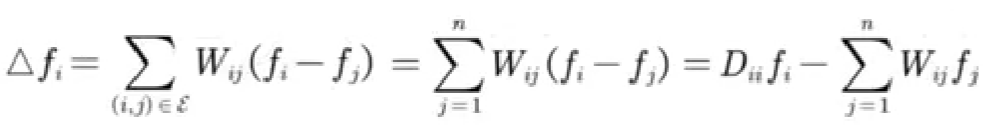
For n nodes there are:

2.2.2 Laplace matrix

A Laplacian matrix is ​​a type of Laplacian operator on a graph.

D is a degree matrix, and the value on its diagonal is the sum of the weights of all edges starting from the i node (nxn square matrix, which is a diagonal matrix).

The Laplacian matrix (L) is the degree matrix (D) minus the adjacency matrix (W), that is, L = D - W.

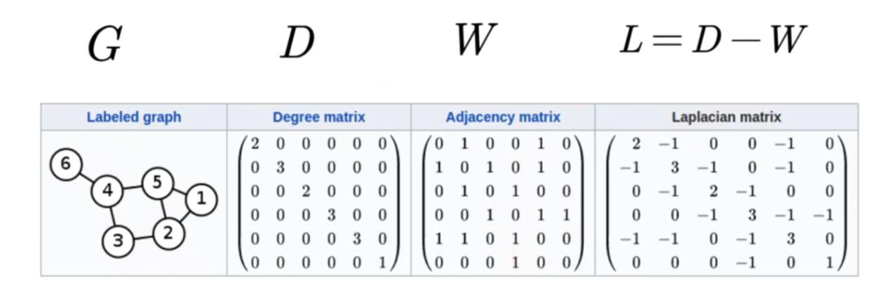
• Properties: The Laplacian matrix is ​​a symmetric positive semidefinite matrix, so the eigenvalues ​​of the matrix must be non-negative, and there must be n linearly independent eigenvectors, which are a set of orthonormal bases in n-dimensional space, forming an orthogonal matrix.

Eigen decomposition, also known as spectral decomposition, is a method of decomposing a matrix into a product of matrices represented by its eigenvalues ​​and eigenvectors.

L is a Laplacian matrix, U is a matrix composed of Laplacian matrix eigenvectors, and λ is a eigenvector, forming a diagonal matrix ∧.

The Laplacian matrix has n linearly independent eigenvectors, which can form a set of basis in n-dimensional linear space.

And because the eigenvectors corresponding to different eigenvalues ​​of the symmetric matrix are orthogonal to each other, the matrix formed by these orthogonal eigenvectors is an orthogonal matrix. So the n eigenvectors of the Laplacian matrix are a set of orthonormal basis in n-dimensional space.

2.3 Graph Fourier Transform

The definition of the signal on the graph: generally expressed as a vector. Assuming that there are n nodes, the signal on the graph is recorded as:
each node has a signal value, and the value on node i isx(i) = xi

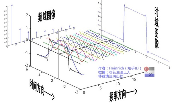
The blue line segment in the figure below represents the size of the signal, which is similar to the grayscale image pixels on the image. The higher the pixel, the longer the line segment drawn.

The classical Fourier transform is as follows

• Fourier Forward Transform F: Find the coefficients of the linear combination. The specific method is to obtain the inner product of the conjugate of the original function and the basis function.
• Inverse Fourier transform f: A signal is superimposed by basis function signals of different frequencies, that is, any function is expressed as a linear combination of several orthogonal basis functions.

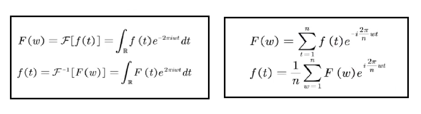
On the left is the Fourier transform in continuous space, and on the right is the discrete Fourier transform.

The essence of Fourier transform is the inner product. Trigonometric functions are a complete set of orthogonal functions. The inner product between trigonometric functions of different frequencies is 0. Only when the inner product of trigonometric functions with the same frequency is not 0.

Refer to an article explaining the essence of Fourier transform, the advantages and disadvantages are clear at a glance

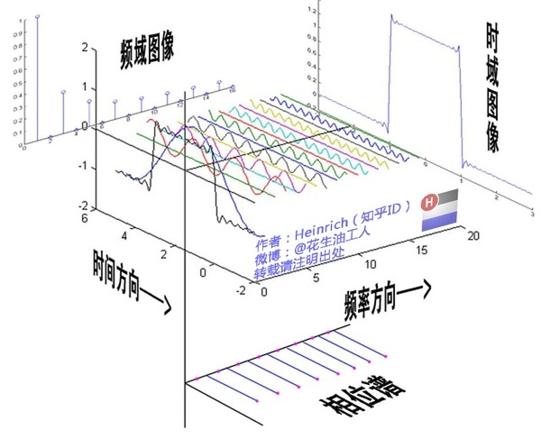
Classical Fourier transform: A signal is superimposed by basis function signals of different frequencies. The red signal in the left figure is the original signal, and the blue signal is the basis function signal (cosine or sine function) at different frequencies. Then the red original signal can be formed by a linear combination of basis functions of different frequencies. The height of blue in the right figure represents the coefficient in front of the basis, which is the so-called Fourier coefficient, which is the coordinate component of the original function on this basis.

The phase is ignored in the figure, the actual Fourier coefficients contain amplitude and phase.

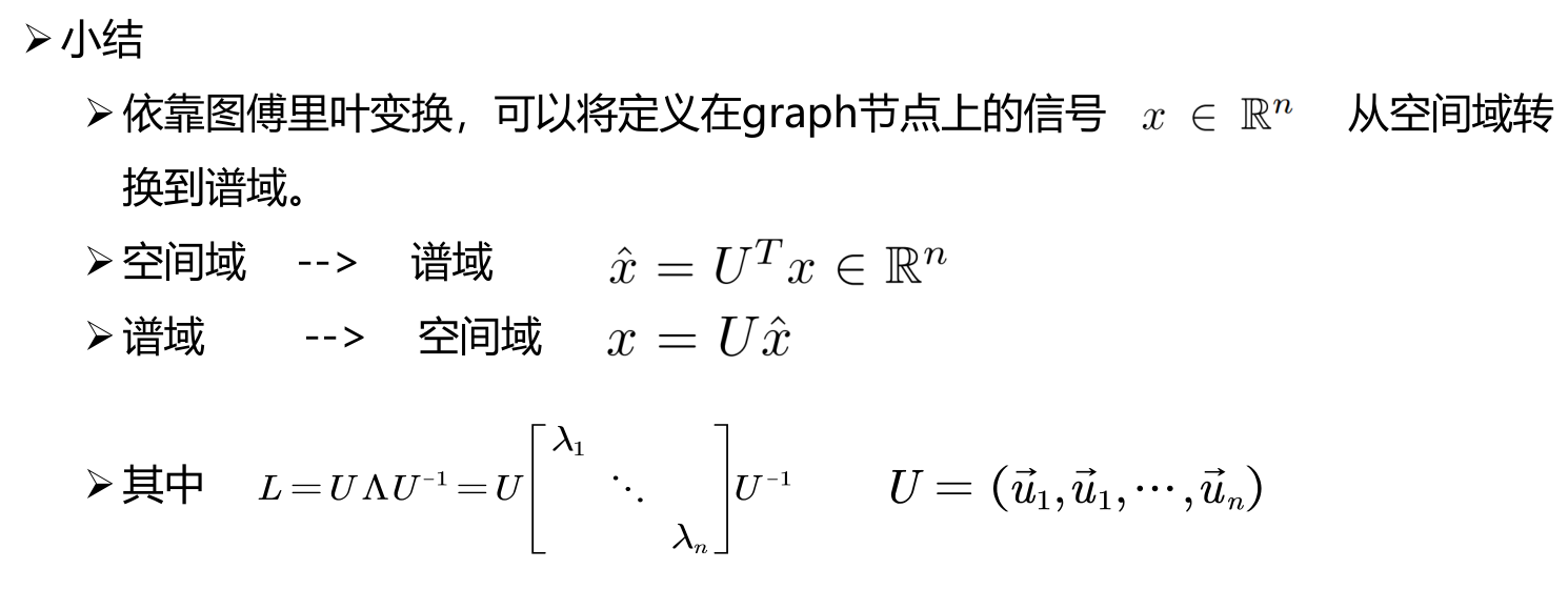
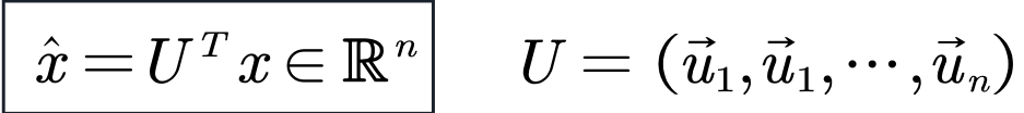
Corresponding to the idea of ​​classical Fourier transform, for the Fourier transform of the signal x on the graph,Hope to find a set of orthogonal bases, and express x through the linear combination of this set of orthogonal bases. The eigenvectors of the Laplacian matrix are just orthogonal, which can be used as the basis function of the Fourier transform of the graph.

Then the inverse Fourier transform can express the signal on the graph as:

Summary: Relying on the graph Fourier transform, the signal x defined on the nodes on the graph can be transferred from the spatial domain to the spectral domain.

Classical Fourier Transform	Graph Fourier Transform
base:	base:
frequency:	frequency":
The amplitude (and phase) of the components:	Amplitude of components:

2.4 Graph Convolution Theorem

The definition of convolution on the figure: first perform Fourier forward transform on the input signal x and the convolution kernel g, and then perform harmand product in the spectral domain, that is, F ( x ) ⊙ F ( g ). Finally, the result is returned to the space domain through the inverse Fourier transform F ^{-1 .}

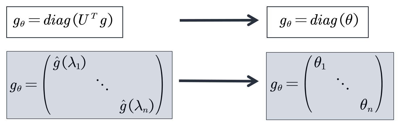
If you express this formula in the form of matrix multiplication, remove the harmand product. At the same time, we usually don't care what the filter signal g looks like in the space domain, but only care about its situation in the frequency domain. Let

the formula be equivalently converted into the following formula:

All spectrogram convolutions follow these definitions, the only difference is the selection of the filter filter

3. Three classic graph convolution models

Introduction

• The three graph convolution models (SCNN, ChebNet, GCN) are all based on the graph theory and come down in one continuous line.
• ChebNet can be seen as an improvement of SCNN, and GCN can be seen as an improvement of ChebNet.
• All three models can be regarded as a special case of the following formula.

Before and after convolution: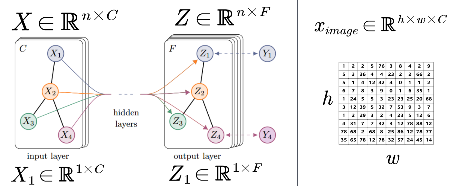
Among them, the feature map of a certain layer can be expressed as an nxc matrix. n means that there are n nodes in the graph, and C is the number of channels. The signals in the graph can be decomposed into signals on each node. X represents the signal on the entire graph, which is a matrix of nxc, and Xi _represents the signal of a certain node, which is a vector of 1xc.

In different layers, the feature map structure does not change, only the signal on the map changes.

---

3.1 SCNN

论文：Spectral networks and locally connected networks on graphs

In the first generation of GCN, two models are given in this paper, which are based on the spatial domain and based on the spectral domain. The core of the spectral domain-based model is to replace the convolution kernel in the spectral domain with a diagonal matrix

main idea:Replacing spectral domain convolution kernels with learnable diagonal matrices, so as to realize the graph convolution operation. Right now:

The formula is defined as follows:

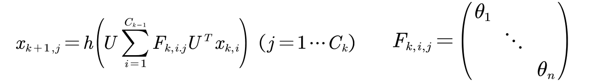
• Among them, C _k represents the number of channels (channels) in the k-th layer, and x _k,i ∈ R ⁿ represents the feature map (feature map) of the i-th channel in the k-th layer
• F _k,i,j belongs to R ^nxn represents the parameterized convolution kernel matrix in the spectral domain. It is a diagonal matrix containing n learnable parameters. h( ) is the activation function.

Disadvantages of SCNNs

• Computing the eigenvalue decomposition of a Laplacian matrix is ​​very time consuming. The computational complexity is O(n ³ ), where n is the number of nodes. When dealing with large-scale graph data (such as social network data, usually with millions of nodes), it will face great challenges.
• The parameter complexity of the model is large. The computational complexity is that it is easy to overfit when the number of nodes is large.
• There is no guarantee of local linkage, because the global linkage is obtained after converting the frequency domain to the air domain.

3.2 ChebNet

论文：Convolutional neural networks on graphs with fast localized spectral filtering

Chebyshev polynomials:

In the matrix state, Chebyshev polynomials can be expressed as:

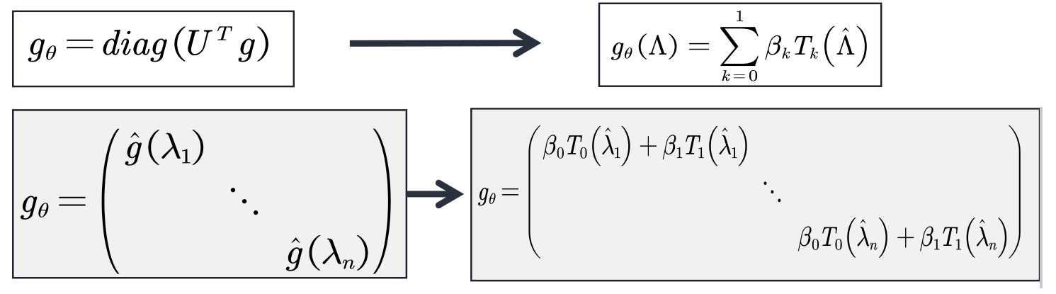
main idea:The filter in the spectral domain is approximated by Chebyshev polynomials.

Because Chebyshev polynomials can be used for polynomial interpolation in approximation theory, that is to say, Chebyshev polynomials can be used to approximate functions.

When fitting, the kth power of x is replaced by the kth order term of the Chebyshev polynomial, and the Chebyshev polynomial is used for approximation. As shown in the figure below:

Why should it be replaced? When replaced, the most time-consuming operation of eigenvalue decomposition of the Laplacian matrix can be omitted in SCNN, and the Laplacian matrix can be used directly.

ChebNet features: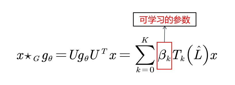

• The convolution kernel has only K+1 learnable parameters, generally K is much smaller than n, and the complexity of the parameters is greatly reduced
• After using the Chebyshev polynomial to replace the convolution kernel in the spectral domain, after derivation, ChebNet does not need to decompose the Laplacian matrix. The most time-consuming steps are omitted.
• The convolution kernel has strict spatial locality. At the same time, K is the "receptive field radius" of the convolution kernel. That is, the K-order neighbor nodes of the central vertex are regarded as neighborhood nodes.

3.3 GCN

论文：Semi-supervised classification with graph convolutional networks

GCN can be regarded as a further simplification of ChebNet: only 1st-order Chebyshev polynomials are considered, and each convolution kernel has only one parameter, so there are only two parameters.

Understanding:

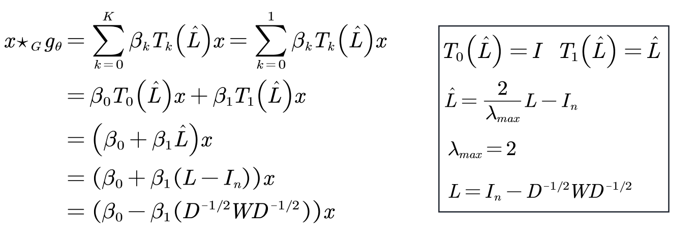
Simplify further so that each convolution kernel has only one learnable parameter.

Because there are eigenvalues ​​in the range [0,2], if this operator is used in a deep neural network model, repeated application of this operator will lead to numerical instability (divergence) and gradient explosion/disappearance. In order to solve this problem, introduce A renormalization trick was adopted.

So as to get the final formula of GCN

Features of GCNs:

• In the case of ignoring the input channel and output channel, the convolution kernel has only one learnable parameter, which greatly reduces the amount of parameters. (According to the author: "We intuitively expect that such a model can alleviate the problem of overfitting on local neighborhood structures for graphs with very wide node degree distributions, such as social networks, citation networks, knowledge graphs and many other real-world graph datasets .”)
• Although the size of the convolution kernel is reduced (GCN only focuses on the first-order neighborhood, similar to the classic convolution of 3X3), the author believes that by stacking GCN in multiple layers, it can still expand the receptive field.
• At the same time, such extreme parameter reduction has also been questioned by some. They believe that if only one learnable parameter is set for each convolution kernel, the ability of the model will be reduced. (You can refer to the blog post How powerful are Graph Convolutions? )
  • If each pixel of a traditional image is regarded as a node of a graph, and there are eight neighbor links between nodes, the image can also be regarded as a special graph. Then in each 3*3 convolution kernel, there is only one learnable parameter.
  • Judging from the deep learning experience currently applied to image, although the complexity of such a convolution model is low, the ability of the model has also been weakened, and it may be difficult to handle complex tasks.