1 Graph Neural Network (Original Version)
The power and use of the graph neural network are gradually being strengthened. I keep writing my views and insights from the most original and now slowly latest papers I have read. I am born in mathematics, so I prefer mathematical derivation. The first article introduces the graph After the beginning of the neural network idea, the graph neural network model is gradually improved based on this.
2 Areas that can be handled
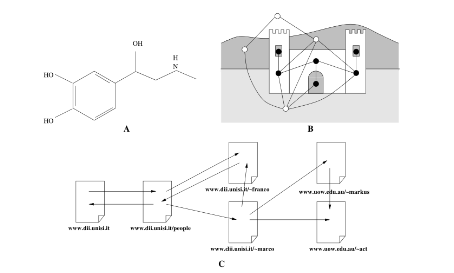
Common unstructured data such as the molecular structure of social networks and other common traveler problems can be processed. The difference lies in how you design g(x), that is, the output function. The contribution of the graph neural model is how to learn an unstructured data and characterize it
3 models
3.1 Introduction
First of all, there are two types of information for graphs: one is graph node information and the other is graph edge information. The nodes of the graph contain the "state" of a node, and we use x(i) to represent the "state" of the i node. This is the model After learning the representation of the graph information, we can intuitively assume the "state" of a point and the state of the surrounding nodes. Using a function f to learn so we can get the following
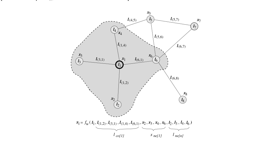
The work we have to do is to learn the "state" of each node in the whole graph, but we will find a problem that the "state" x(i) of the i node depends on the state x(j) of the j node. Similarly The j point is also that the two constantly depend on each other to form a cycle. The assumption of the model is that we can solve the "state" of the whole graph through loop iteration
3.2
We introduce our output function g(x,l) that the output of a node will be related to the "state" of this point and the connected edges
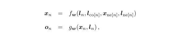
From this we get two functions of our overall model, one to solve the state of the graph and one to output (according to the actual task)
The key we need to solve is how the f function solves the state of the entire graph. There is a mathematical theory that when the derivative of f to x is less than 1, we can guarantee convergence 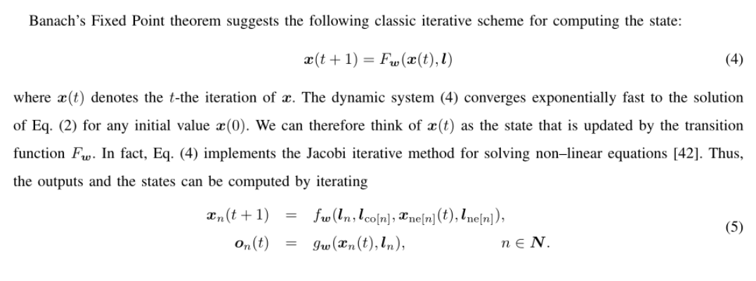
In simple terms, the iterative process is to update the state of the t+1 round with the state of the t round, and finally obtain the state of the full graph convergence.
3.3

So now we can expand the solution process in rounds, where g and f are both neural network structures and you can design them yourself. We expand the entire solution process into the following form, in which the front is the state process of the continuous iterative solution graph 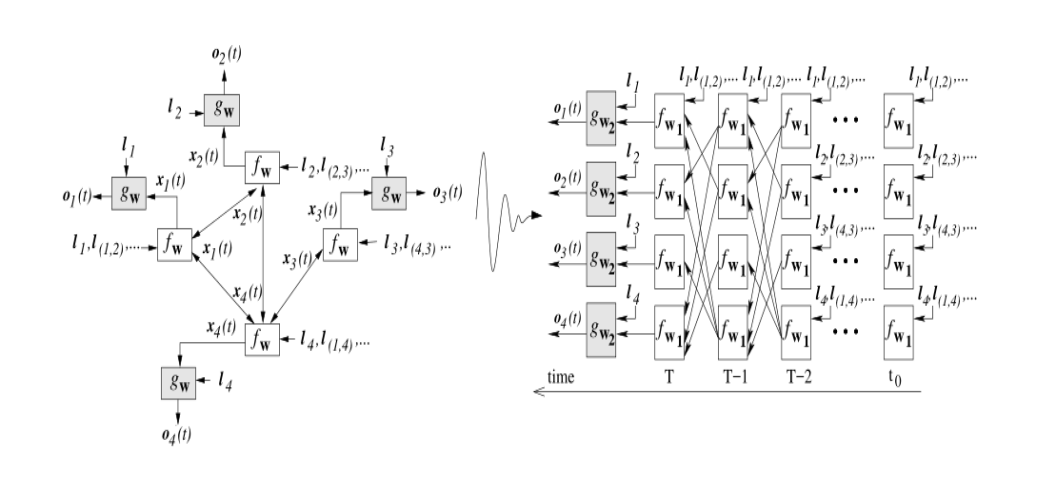
3.4
The general idea of the graph neural model was introduced earlier. Next, I will introduce the gradient descent and the derivation process. Because the graph neural network needs to ensure that the state converges in the solution process before it can proceed to the next step, the iterative process of derivation is different.
First we introduce the existence of an implicit function
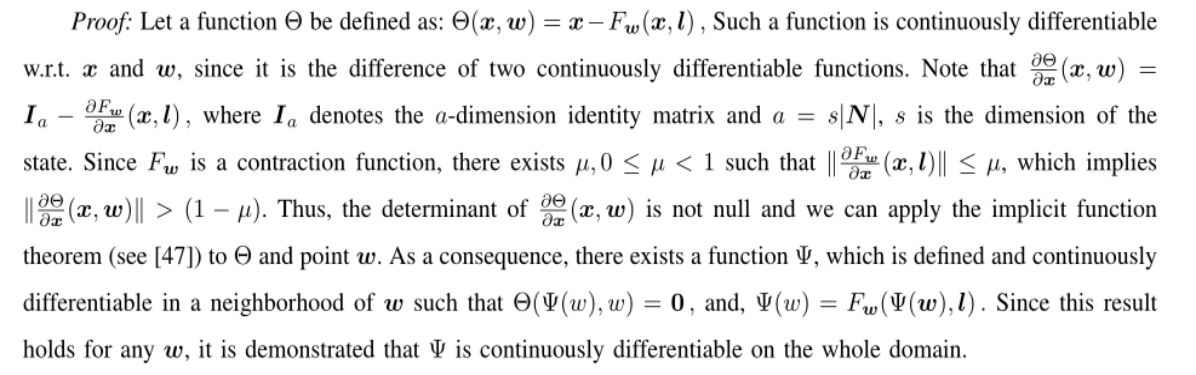
This function reflects the distance between the state x we really need and the x(t) of the t round we are looking for. It can theoretically prove that there is a parameter w that allows us to solve the perfect x, and then connect the parameter w to x .
3.5
Then when we introduce our loss function e, how to define the loss is closely related to your output function g, and you need to design it yourself. According to the model expansion structure, we get the following derivation formula 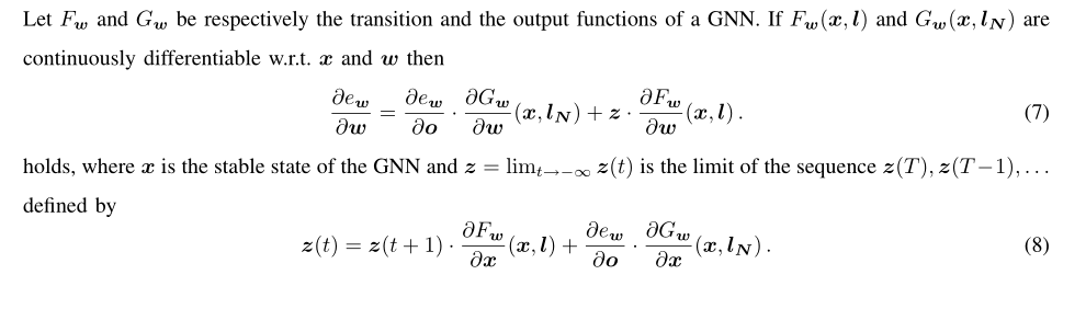
This derivation rule for passing time is very close to traditional rnn and I will not repeat it. According to our assumption, z(t) is equal to z(t+1) after a certain number of iterations 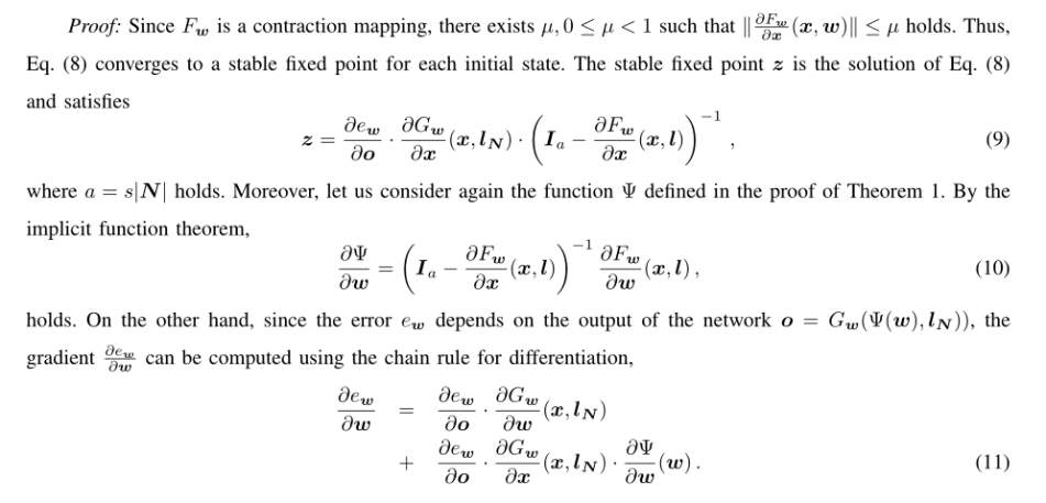
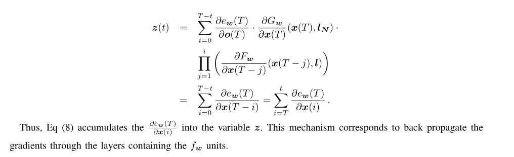
According to (8), we get (9) We then obtain (10) according to the implicit function we have proved before, and according to the implicit function derivation rule, (11) to solve the derivative for the other direction is not based on the expansion of our model, but directly based on the partial The derivation definition directly obtains the result and brings (9) (10) (11) into the following derivation rule 
Again, all the derivation formulas are transformed into the derivation of the parameter w. Next, an iterative process of z(T) is similar to the summation of a sequence of numbers. 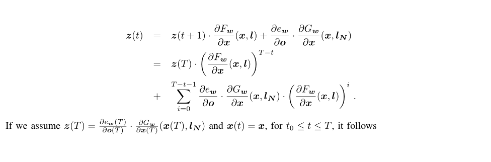
So far we have all our derivation rules
3.6 Model Algorithms
In the derivation process, we assume that when we converge to a value, we can use the formula we derived for derivation. Therefore, in terms of the algorithm, we need to add two steps to verify the convergence and then continue the derivation. The overall algorithm block diagram is as follows 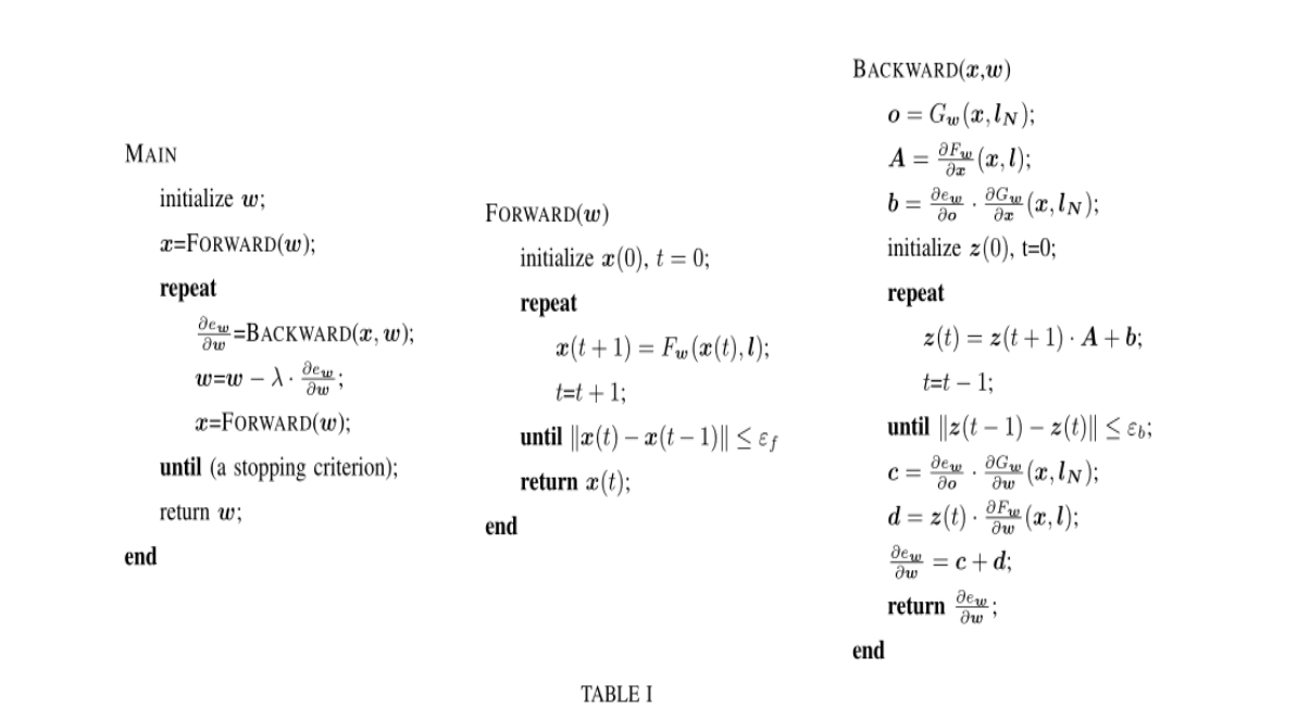
4 Summary
The contribution of the overall model is to solve the problem of how to learn the characteristics of an unstructured data, using the method of iteration to the convergence value to learn, maybe everyone has also discovered that this model does not focus on the current relationship between the two points. The graph neural idea is similar but with the addition of edge learning.
5 Questions and thoughts
First of all 1) In the calculation process of this model, it is necessary to ensure that the derivative of f to x is less than 1. This will prevent the model from deepening the number of layers. When the number of layers is high, problems such as gradient disappearance will inevitably occur.
2) There is no effective learning edge information