Hand tear graph machine learning, graph neural network

A neural network is a very powerful tool that can handle different types of data in different modalities. In the NLP series of articles , the use of cyclic networks in sequence data (articles are mainly text information, because audio information processing has not been involved too much, so no summary is made), including related explanations and explanations of Transformer and attention mechanism application. In the Gephi tutorial , the graph drawing and some graph analysis and visualization based on the Gephi software are introduced. Gephi just opened the tip of the iceberg for graph analysis. In fact, we don't have enough tools to mine and interpret the information behind the graph. Graph analysis is also a kind of sequence information, but this sequence information is more about correlation and causal inference. Therefore, the analysis of graphs can be independent of the direction of NLP, as a new direction to explore and learn. This article will mainly summarize relevant theoretical content about graph machine learning and deep learning as a supplement. In addition, due to the huge workload of code implementation, another document will be created to organize the code, and a hyperlink will be attached to the supporting notes , which can be read on demand. Since the knowledge of graphs will involve a large number of graph theory and matrix-related operations, after the end of this article, a new document will continue to be opened to sort out related mathematical content. Intensive reading of related classic algorithm papers will be used as supplementary content of graph series articles .

手动防爬虫，作者CSDN：总是重复名字我很烦啊，联系邮箱daledeng123@163.com

1. Why?
In the traditional field of machine learning, the relationship between data sample A and data samples B, C, and D is not taken into consideration. We default these parameter variables as independent and identically distributed variables that have nothing to do with each other. Of course, a similarity matrix can also be used to describe the similarity and correlation between these variables, but this is not the original intention of machine learning. The graph is just a common language for describing such data relationships, and more related information can be mined by using the graph information.

2. How?
Make full use of the relationship between Node and Edge for data mining. If you want to use the network to process graph data, you first need to be clear that the input data size of the graph is not fixed, and a Node may form a relationship with N points, and this N can be extremely huge and unlimited data. For image data (convolutional network) processing, the convolution process of the convolution kernel is a scanning process from left to right and top to bottom; for text data (circular network) processing, it is also a calculation from left to right Process; for graph data, there is no initial anchor point, and it has multi-modal characteristics. For example, the popularity of a certain music may be related to composers and singers (text data), it may be related to audience portraits (text data), and it may be It is related to whether the MV is good-looking and the rhythm is dynamic (audio data), and it may be related to whether the album cover is good-looking (image data). Therefore, graph data processing is essentially a combination of various convolution operations, regularization operations, supervised learning operations, etc. that turn node information into a d-dimensional vector of end-to-end learning. This process is called graph embedding. ), figuring out how to do a good job in gragh embedding is as important as doing a good job in word embedding in NLP.

3. Application
(1) The shortest path (graph theory problem).
(2) Node importance analysis (degree centrality evaluation).
(3) Community detection (find important groups that share similarities among broad groups).
(4) Similarity and association prediction (there may be connections between nodes that are far apart).
(5) Joint effect detection (if there is a great possibility of combination, beyond the ability of clinical medical detection, the graph can find the potential correlation of these nodes, such as a+k has not been clinically verified, the graph analysis a+ k is beneficial to clinical performance).
(6) Graph embedding problem (the core of establishing connection with deep learning).

Written in front & supporting link (visitors must read)

The text explains the principles of graph network and graph learning in easy-to-understand language. It will involve some simple mathematical inferences. The complete mathematical inferences of the key conclusions will be written as a supplement when I have time later. All the graphs involved in this article The feature description method can be implemented with relevant codes. The current mainstream graph mining toolkits include Gephi, NetworkX, PyG, and Gephi is an integrated software installed locally on the computer. It has built-in graph drawing, graph visualization, and some simple clustering analysis functions. Great for getting started. NetworkX is a set of graph analysis tools based on statistics and topology. It is easy to install, has complete documentation, and has a certain degree of data mining and analysis capabilities. It is suitable as a tool for getting started with graph machine learning. PyG is a graph neural network tool based on pytorch. It integrates the mainstream graph mining neural network framework. It has multi-modal and multi-dimensional mining capabilities for graph information. It is a very powerful graph analysis tool, but requires a certain GPU. Resources, suitable for advanced selection. Since the relevant content is still being updated non-stop, the supporting links may not be complete, and will be added later. The workload is heavy, so please do not send private messages to remind me to update
my personal feelings after learning: In fact, the core of graph mining is still the NLP method, but it weakens certain sequence perception and strengthens topological structure cognition, which coordinates time and space A set of model methods for dimensions, from the perspective of learning, NLP is still prioritized over GNN.
NLP starts from 0 (mainly see the idea of ​​Word2Vec in the coding chapter)
Gephi graph visualization tool uses
the code of NetworkX basic operations and graph analysis-related calculations
[Paper intensive reading series, the pioneering work of graph machine learning towards graph deep learning] DeepWalk, random walk The art of graph embedding, the first integration of natural language processing and graph processing
[Handwritten code reproduction] DeepWalk actual combat

Basic representation of graph

Basic parameters of graph

Nodes: nodes/vertices $Side\; N$
: links/egdes$E$
system: network/graph$G(N,E)$

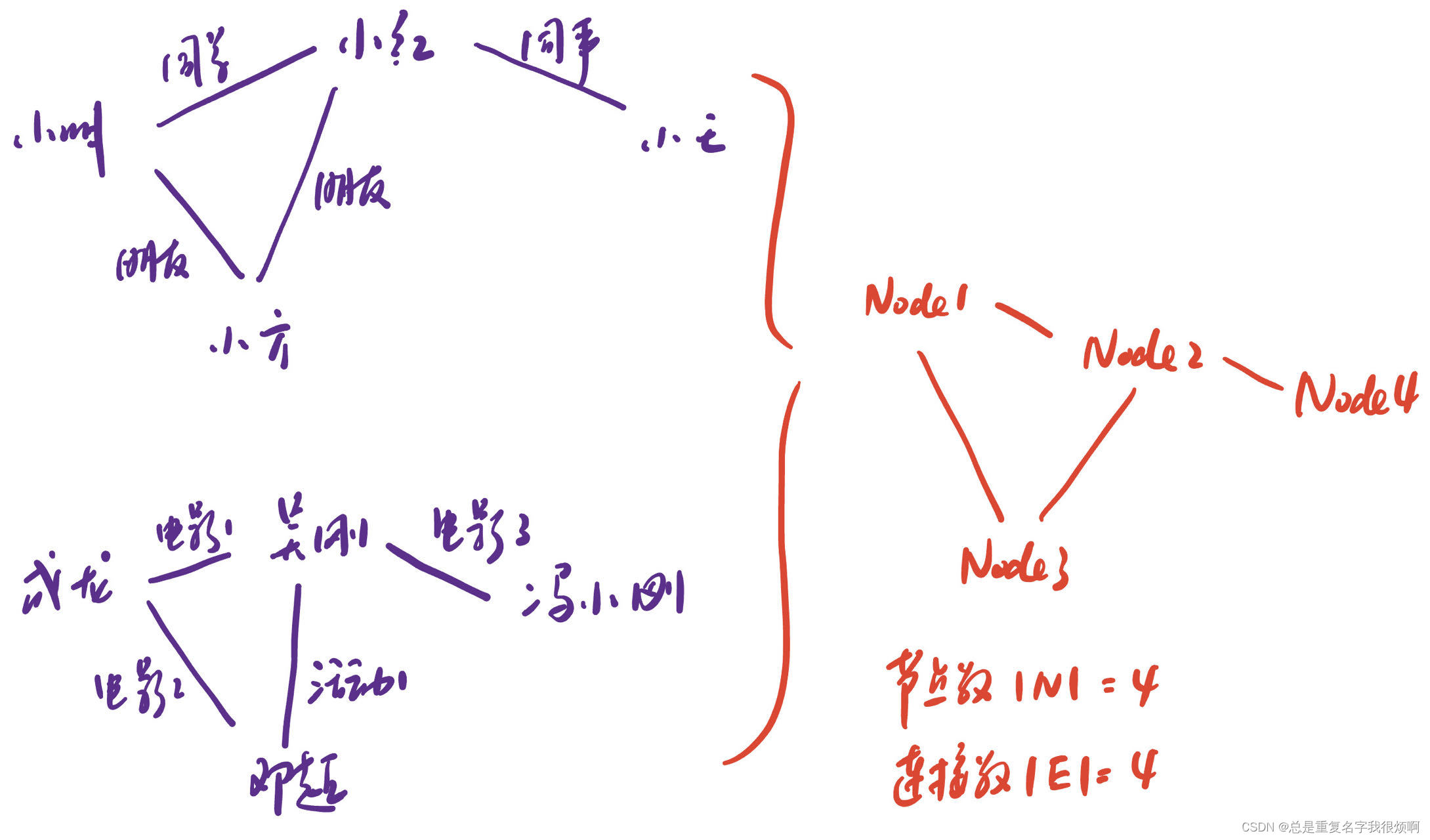
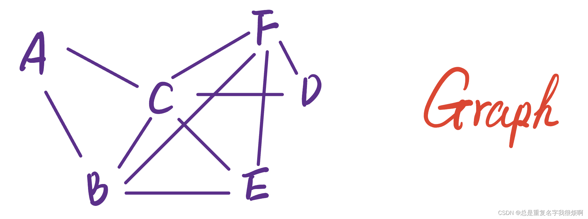
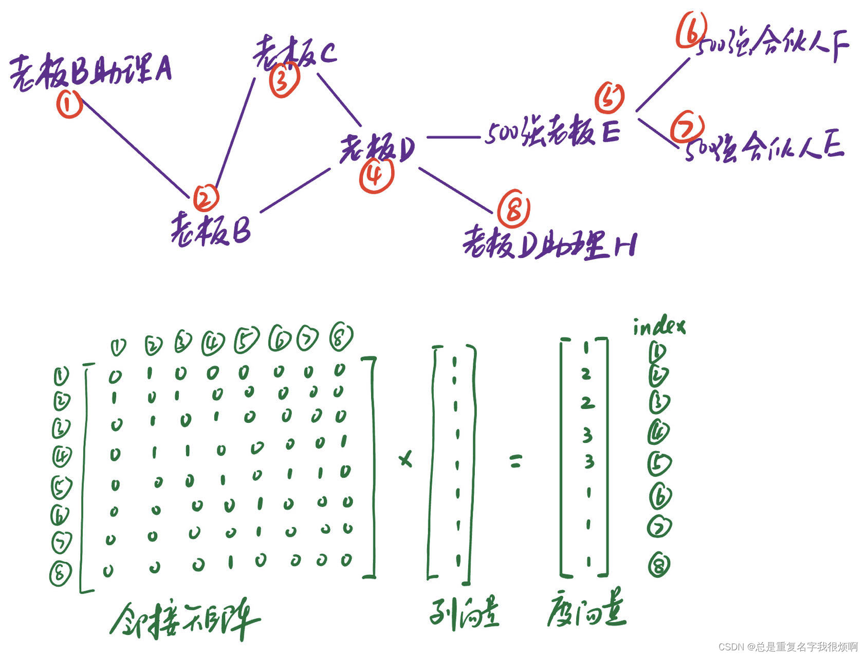
For example, these two infographics can essentially be drawn as one graph (number of nodes 4, number of connections 4). In fact, the design of the graph needs to be determined according to the actual relationship you want to solve the problem.

class of graph

There are undirected graphs and directed graphs.
For the type of relationship, it can be divided into n-dimensional heterogeneous graphs.
$$\begin{gathered} G=(V,E,R,T) \\ {v}_i\in V,\; environmental\; factors\; such\; as\; blood\; pressure,\; disease,\; age,\; gender,\; etc. \\ (v_i,r,v_j)\in E,\; the\; combined\; effect\; of\; these\; environmental\; factors \\ edge\; relationshipr\in R \\ Node\; categoryT \end{gathered}$$
The most common heterogeneous graph of$$node\; category$$$$T\; is\; a\; bipartite\; graph\; (2\; kinds\; of\; nodes,\; bipartite\; graph).$$Such as the relationship between work and names, authors and titles of published papers, etc. Such bipartite graphs can be expanded directly.

Number of Node Connections (Node degree)

For paper2 in the above figure, the number of connections of nodes is 3, recorded as $k_{paper}=3$
degree of tie$k_{avg}=<k>=\frac{2E}{N}$
If it is a directed graph, there is no node sharing. At this time, the tie degree $k_{avg}=<k>=\frac{E}{N}$
We can describe the importance of nodes with node degree

Matrix representation of a graph (adjacency matrix)

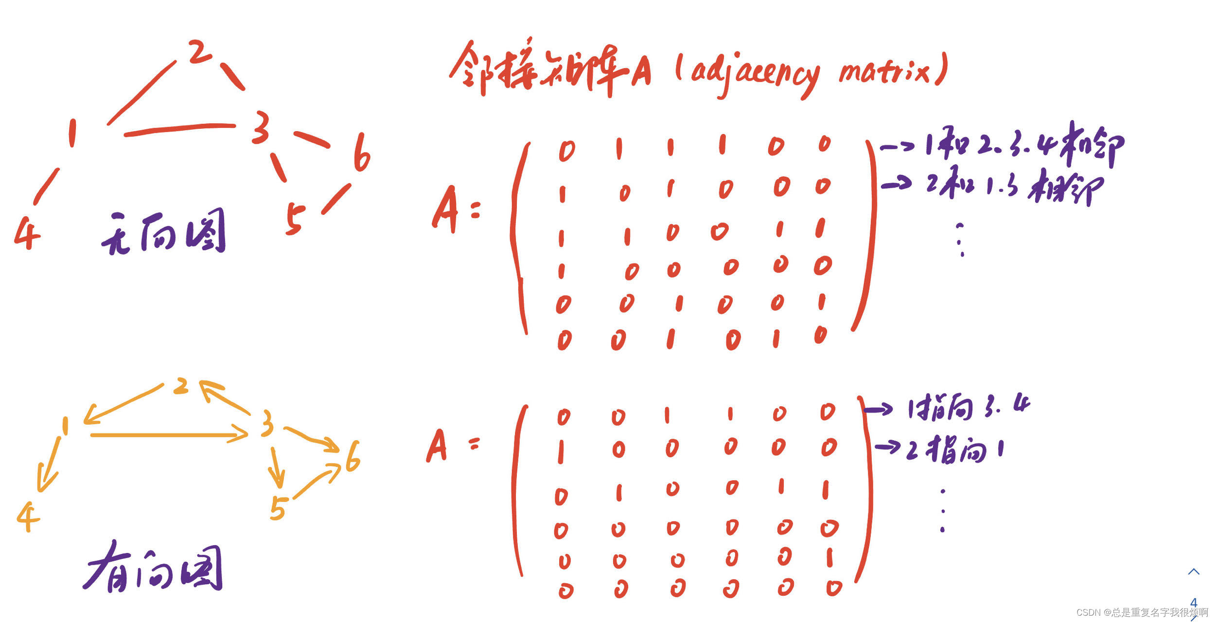
For an undirected graph, its adjacency matrix is ​​a symmetric matrix, and an undirected graph is an asymmetric matrix. In mathematical language:
$$A_{ij}=1，ifthereisalinkfromnodeitonodej,else0$$
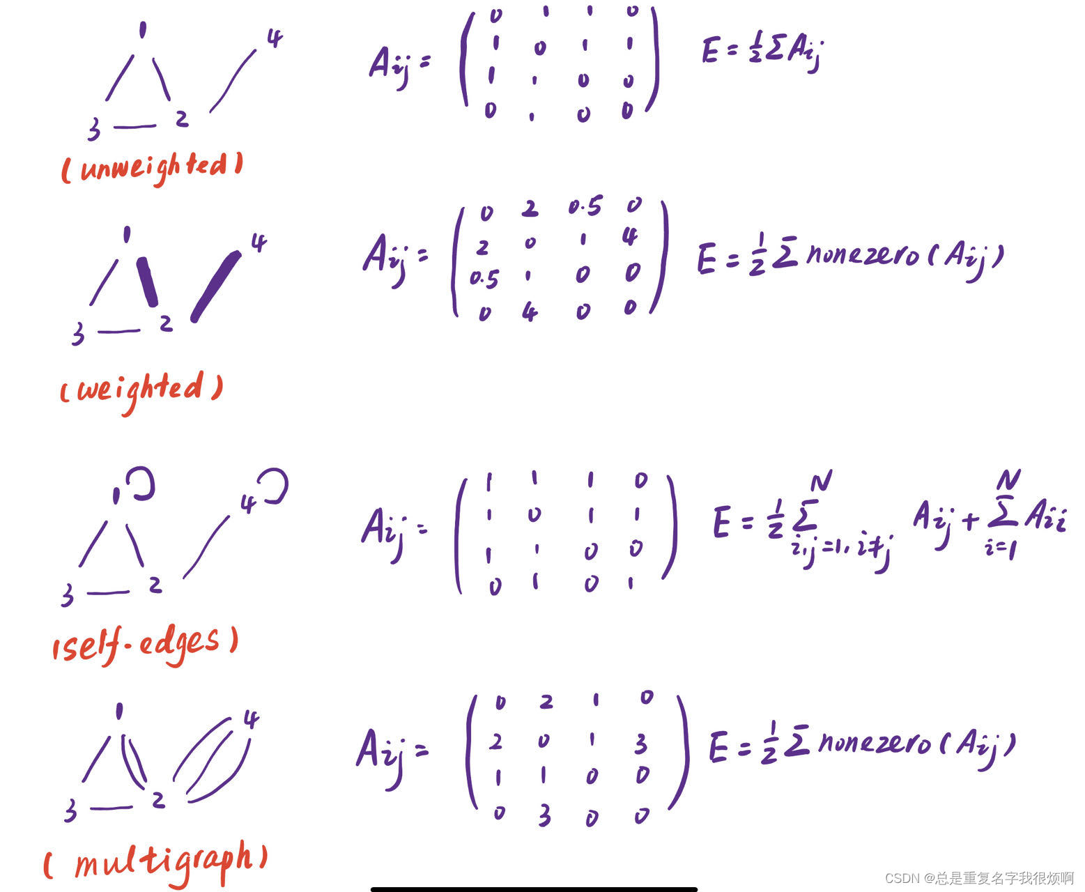
Since the adjacency matrix of an undirected graph is a symmetric matrix, the total number of connections$L=\frac{1}{2}\sum A_{ij}$. The total number of connections $L=\sum A_{ij}$

Thinking 1: Why should the graph be expressed in matrix form?
Thinking 2: The seemingly perfect adjacency matrix is ​​mostly a sparse matrix in reality.

Link List and Adjacency List

Connected list: Only record the list where there are connected node pairs. The directed graph above can be recorded as: (1, 3) (1, 4) (2, 1) (3, 2) (3, 5) (3, 6) (5, 6) adjacency
list: only record adjacent nodes. The directed graph above can be recorded as: (Only 4 lines are used to represent graph information)
1: 3, 4
2: 1
3: 2, 5, 6
4:
5: 6
6:

other pictures

Traditional graph machine learning (feature engineering + machine learning)

The graph has three layers of information that can be written in the form of vectors: (1) node information; (2) connection information; (3) region information. However, the attributes contained in the node information are often in the form of multi-modality, such as the person's avatar (image information), personalized signature (text information), and so on. However, it is difficult for machine learning to deal with multimodality, so traditional machine learning mainly mines the connection feature information between nodes, such as what role this node plays in the entire community.

How to do graph feature engineering (node ​​level)

To put it simply, what to do in this part is to use all the node information to guess the information of unknown nodes, such as using the categories of all nodes in the Chengdu subway network to guess whether Moziqiao Station may be a subway station. The method is to edit the node information into a D-dimensional vector, and then import the algorithm for calculation.
$$\begin{gathered} G=(V,E) \\ f:V\to R \end{gathered}$$
inputs the D-dimensional vector of a certain node, and outputs the probability that the node is a certain class. The key to this is how the D-dimensional vector is constructed.
Generally speaking, the following four information can be included in traditional machine learning: (1) node degree, degree (2) node centrality, importance (3) clustering coefficient, aggregation coefficient (4) graphlets, subgraph splitting

Node degree centrality - single similarity

Described by connectivity alone, it can only explain the similarity of a single dimension, and cannot cover more information, such as 1 and 7, obviously their quality is different, but the node degree is 1. So other importance metrics are needed to further describe graph information. (The degree vector here is actually node degree centrality)

Eigenvector centrality (eigenvector centrality) - birds of a feather flock together

This is a very conventional idea: if a node and its adjacent nodes are both important, then this node is also important.
We use $c_v$Indicates the importance of node v, at this time the importance of this node is:
$$c_v=\frac{1}{l}\sum c_u$$where $\lambda$ is the largest eigenvalue of the adjacency matrix,$c_u$is the importance of v adjacent nodes. That is, the importance of v's adjacent nodes is summed and then normalized to obtain the importance of v's nodes.
Then this problem becomes a classic recursive problem. In this case, eigenvectors can be used to solve it.
$$c_v=\frac{1}{l}\sum c_u\equiv \lambda \mathbf{c}=Ac$$
where A is the adjacency matrix. We can understand such a process in terms of the rank of the matrix. Assuming that the v node is adjacent to 4 nodes, for the left side$\lambda c$ is a 4x1 matrix, for the right side, the adjacency matrix A is a 4x4 matrix, c is a 4x1 matrix, their result is still a 4x1 matrix.
$$l{\left[\begin{array}{c}a\\ b\\ c\\ d\end{array}\right]}_{4\ast 1}={\left[\begin{array}{c}0a_{12}{a}_{13}{a}_{14}\\ b_{11}0b_{13}{b}_{14}\\ c_{11}{c}_{12}0c{}_{14}\\ d_{11}{d}_{12}{d}_{13}0\end{array}\right]}_{4\ast 4}{\left[\begin{array}{c}a\\ b\\ c\\ d\end{array}\right]}_{4\ast 1}$$
In this case $c$ is the eigenvector of A. And, this$c$ is the eigenvector centrality we need to obtain.

Betweenness centrality - the center

This importance index is mainly used to measure whether the node is in the center. For example, Mayday Beijing concert, then Mayday must be at the center of all connections. The calculation method of inter-importance is as follows:
$$c_v=\sum \frac{How\; many\; pairs\; of\; nodes\; have\; the\; shortest\; path\; through}{Number\; of\; pairs\; of\; pairwise\; nodes\; other\; thanv-\; nodes}$$
To better illustrate with an example:

From the inter-importance, it can be found that C and D are in the position of the traffic arteries in the whole graph, and although B is adjacent to CD, the importance of B is obviously not as high as CD.

Shortest path importance (closeness centrality) - close to everywhere

The importance can be calculated by the following formula.
$$c_v=\sum \frac{1}{The\; shortest\; path\; fromnodevto\; other\; nodeu}$$
Also use the image above as an example. The shortest path importance of node A is:
$$c_a=\frac{1}{2+1+2+3}=\frac{1}{8}$$
The node path length is divided into ACB (2), AB (1), ACD (2), ACDE (3). The
shortest path importance of node C is:
$$c_c=\frac{1}{1+1+1+2}=\frac{1}{5}$$
The node path length is divided into CA (1), CB (1), CD (1), CDE (2)
because $c_c>c_a$, so the importance of point c will be higher than that of point a, which means that point c is close to everything, and point a has a sense of suburbia.

Clustering coefficient (clustering coefficient) - hold together for warmth

$$e_v=\frac{}{Pairwise\; pairs\; of\; adjacent\; nodes\; ofv\; node}$$

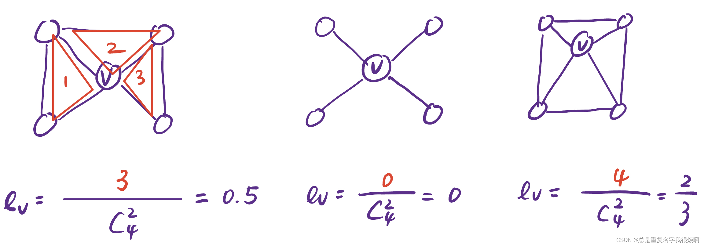
will find the third $e_v$greater than the first $e_v$, indicating that for the v node, the third group will be more serious. This kind of center links out, and the connected points can form a new network. This kind of network can also be called an egocentric network.

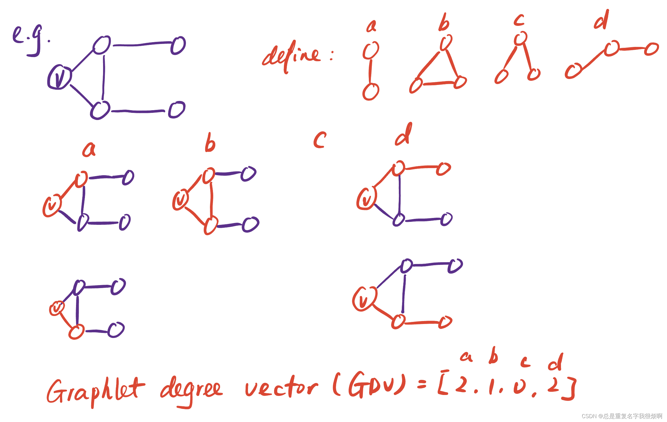
subgraph vector (graphlet degree vector)

We can represent the local neighborhood topology of node v through some topological structures defined by ourselves. It is equivalent to constructing a histogram, and then making a respective description of the node roles defined by oneself. Further, GDV can be used to calculate the similarity of nodes and the like. If the number of nodes we define is 5, then there will be 73 topological structures. In this case, GDV is a 73-dimensional vector. In this case, the description of the topological information of the nodes will be more comprehensive.

some thinking

No matter how the importance between nodes is described, only the graph information of nodes can be described, but the attribute information of nodes cannot be described. In this case, even if the feature engineering is the best, it is difficult to achieve community classification. For example, there are three identical graphs, and they belong to Chaoyang District, Haidian District, and Xicheng District. In this way, it is very difficult Divide them into three categories, and achieve the ultimate feature engineering, the more consistent the information expressed by the three, the greater the possibility of being divided into one category. This is the downside of machine learning. Therefore, in the case of unlimited computing power, it is the most feasible way to describe the graph by considering as many dimensions of information as possible.

How to do graph feature engineering (connection level)

In this part, we need to express the connection between nodes as a D-dimensional vector, and realize the prediction and analysis of unknown connection information between nodes through the connection information between nodes. So the key is how to extract this D-dimensional vector.

Idea 1: Directly extract link information into a D-dimensional vector
Idea 2: Splicing the node information at both ends of the link into a D-dimensional vector
is actually the same as the previous node information mining, and the connection structure information will be lost, such as boss A and The node information of employee A cannot represent the connection information of such an affiliation relationship between the boss and the employee. Therefore this method is not recommended.

shortest path distance

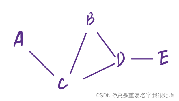
Here, the shortest path lengths from A to B, B to E, and C to E are all 2, but it can be found that if CD is a point with a high weight, the quality of the two connections ACB and ACD is different . Therefore, only focusing on the distance length will lose quality information.

neighborhood relationship

(1) Common neighbors (the number of common friends).
$$|N(v_1)\cap N(v_2)|$$
（2）Jaccard's Coefficent（交并比）
$$\frac{|N(v_1)\cap N(v_2)|}{|N(v_1)\cup N(v_2)|}$$
Take the above figure as an example, the intersection of AB nodes is C, and the union of AB nodes is CD, then the intersection and union ratio of AB nodes is $\frac{1}{2}$。
（3）Adamic-Adar index
$$\sum _{u\in |N(v_1)\cap N(v_2)|}\frac{1}{log(k_u)}$$
Take the above picture as an example, the common friend of node AB is only C, at this time the Adamic-Adar index is $\frac{1}{log3}$. Generally speaking, if the common friend of two nodes is a common point (similar to Sheniu or Neptune), then the connection between the two nodes is not so strong. For example, Xiaoming and Xiaohong are both in Sichuan University, then Xiaoming and Xiaohong Red does not necessarily produce too much intersection. Conversely, if the mutual friend of the two nodes is a social terror, for example, Xiao Ming and Xiao Hong both know Xiao Wang of the research group. Then the connection between Xiao Ming and Xiao Hong will be stronger. At this time, if Xiao Wang is a reclusive person who lives in the laboratory all year round, then there is a high probability that Xiao Ming and Xiao Hong will be more in love than Jin Jian.

Thinking (Katz Index)

If the two nodes have no common friends, then the number of common friends and the ratio of cross-union are all 0 at this time, but in fact there may be a certain connection between the two nodes. Therefore, in this case, you need to see the full image information. It is often represented by the Katz index, which represents the number of paths of length k between node u and node v. The katz index can be calculated using the power of the adjacency matrix.

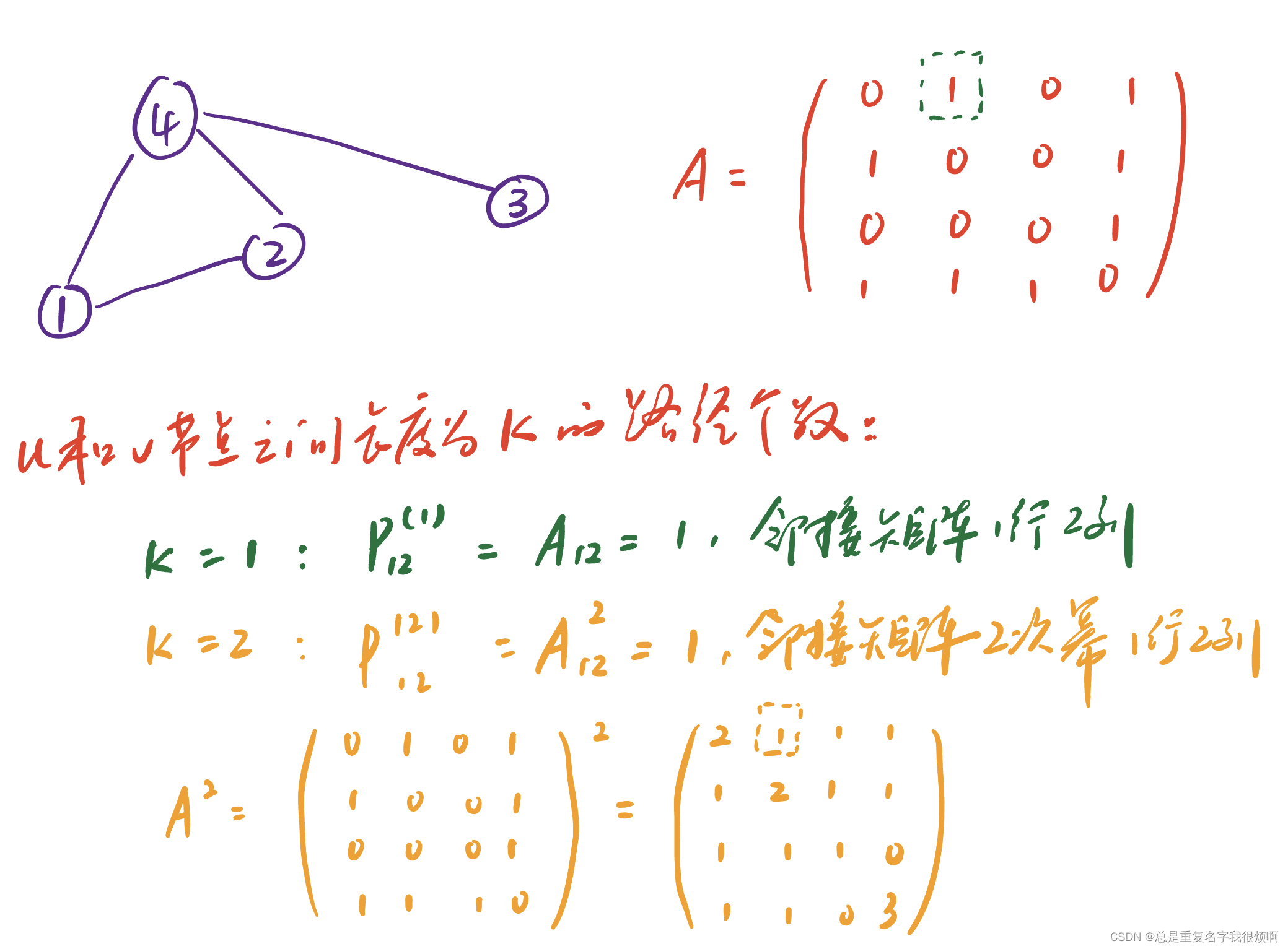
proof:
$$P_{uv}^{(2)}=\sum _i{A}_{ui}\ast P_{iv}^{(1)}=\sum _i{A}_{ui}\ast A_{iv}=A_{uv}^2$$
Understanding:
$A_{ui}$Indicates that the neighbor i is 1 step away from node u, $P_{iv}$Indicates whether i is 1 step away from u. Still use node 12 as an example, at this time u=1, v=2, $A_1$Indicates the node that is one step away from node 1, that is, nodes 2 and 4, the adjacency matrix is ​​the first row vector of [0 1 0 1], P i 2 P_{i2 $P_{i2}$At order 1 is equivalent to $A_{i2}$Yes, the adjacency matrix is ​​the second column vector of [1 0 0 1]. Here, i and u are separated by 1 step, and i and v are separated by 1 step. In fact, u and v are separated by 2 steps.

继续证明：
$$\begin{gathered} P_{uv}^{(2)}\equiv A_{uv}^2 \\ {P}_{uv}^{(3)}=\sum _i{A}_{ui}\ast P_{iv}^{\left(2\right)}=\sum _i{A}_{ui}\ast A_{iv}^2=A_{uv}^3 \\ \dots \dots \\ {P}_{uv}^{(l)}=A_{uv}^l \end{gathered}$$

Further, this length can be added to infinity (1, 2, 3, ..., ∞). Then the sum of all path lengths of nodes v1 and v2 is:
$$S_{v_1{v}_2}=\sum _{i=1}{b}^i{A}_{v_1{v}_2}^i$$
Here, $\beta$ is a reduction factor, usually$0<b<1$ . The greater the length, the greater the reduction.
Actually,$S={\sum }_{i=1}{(\beta A)}^i$ is the sum of a geometric sequence, which can be expanded by geometric progression.
$$S=\sum _{i=1}{\left(\beta A\right)}^i=(I-\beta A{)}^{-1}-I$$
against this formula progression one proof:
$$\begin{gathered} (I+S)(I-\beta A) \\ =(I+\beta A+b^{2A}{\_}^2+\cdots +b^A{\_}^n)(I-\beta A) \\ =I+\beta A+b^{2A}{\_}^2+\cdots +b^A{\_}^n-(\beta A+b^{2A}{\_}^2+\cdots +b^{n+1}{A}^{n+1}) \\ =I \end{gathered}$$
factor this:
$$S=(I-\beta A{)}^{-1}-I$$

How to do feature engineering of graphs (full graph level)

From BoW to BoN

This part needs to extract a D-dimensional vector to describe the characteristics of the entire image. When NLP did not enter the transformer period, it was still in the stage of machine learning (N-Gram), and faced the same problem, that is, how to convert textual information into vector information and input it into the computer. At this time, a very great idea was proposed (bag-of-words, BoW). The core of this idea is to count the number of occurrences of a certain word or word in a piece of text, and then encode it into a vector form, for example, "I love you and you love him", this sentence I and him appeared once, love you appears 2 times, then this sentence can be encoded as [1,2,2,2,2,1]. Of course, this encoding method is rough and has many problems, and it does not consider word segmentation, so there are many problems, but this idea realizes a key step in the conversion of text information to tensor information. By the way, let me promote the previous articles. If you want to learn more about NLP related content, you can read the NLP series of articles in my blog. NLP starts from scratch .
Based on the idea of ​​BoW, we can regard the nodes of the graph as words and propose a bag of nodes (BoN) idea.
$$\varphi (G_1)=[nodes1number,nodes2number,\dots ]$$
Of course, this way of thinking also has many disadvantages. The most fatal point is that it only has node information and no connection information, so it needs to be further upgraded on this idea.

From BoN to BoND

Only look at the number of node degrees, not the number of nodes or connections.

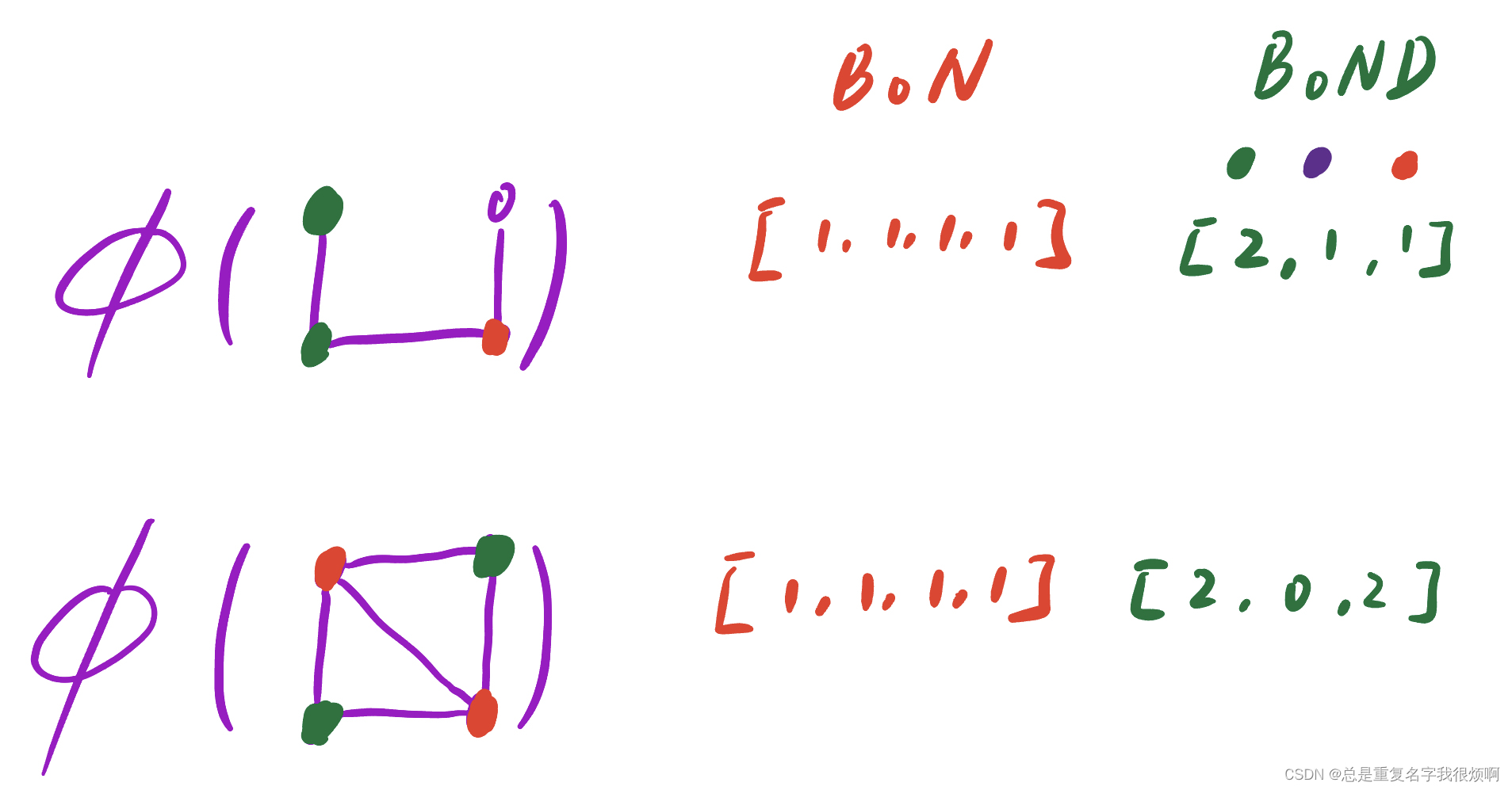
If the idea of ​​BoN is used, the vector representations of the two graphs are the same, and each point appears only once (the four nodes are not the same). If the idea of ​​BoND is used, the two graphs can be distinguished.

BoG（bag of graphlet）

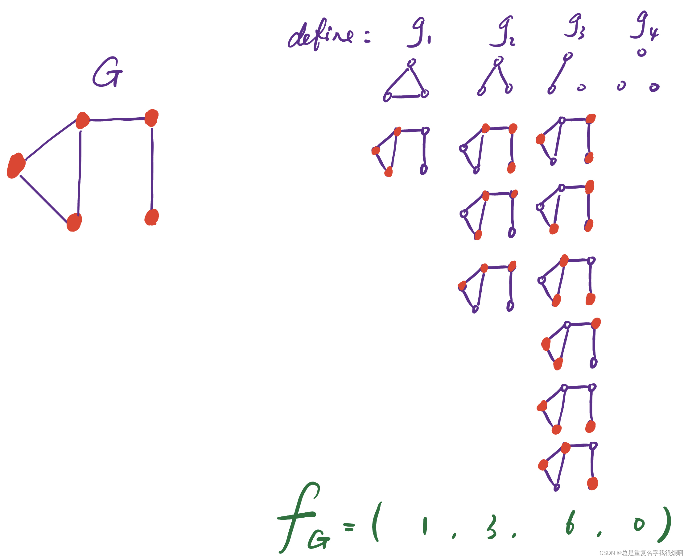
At this time, if $f_G$Do the quantity product, that is, $K(G,G^{\prime })=f_G^T{f}_{G^{\prime }}$, which can reflect the similarity between the two graphs. Of course, if the numbers of the two maps are very different, for example, one is the Beijing subway network and the other is the traffic flow network in the Ali area, then even if they are similar, the product of the numbers will be very large. Therefore, generally need to $f_G$Do a normalization process.
$$\begin{gathered} h_G=\frac{f_G}{\sum f_G} \\ K(G,G^{\prime })=h_G^T{h}_{G^{\prime }} \end{gathered}$$

But if there is a huge network graph with n nodes, it is very uneconomical to do this k-size subgraph matching calculation, because it is necessary to perform subgraph matching on the nodes of the whole graph, and the computational complexity is nkn $n^k$

BoC（Weisfeiler-Lehman Kernel）

This is a method based on color refinement.

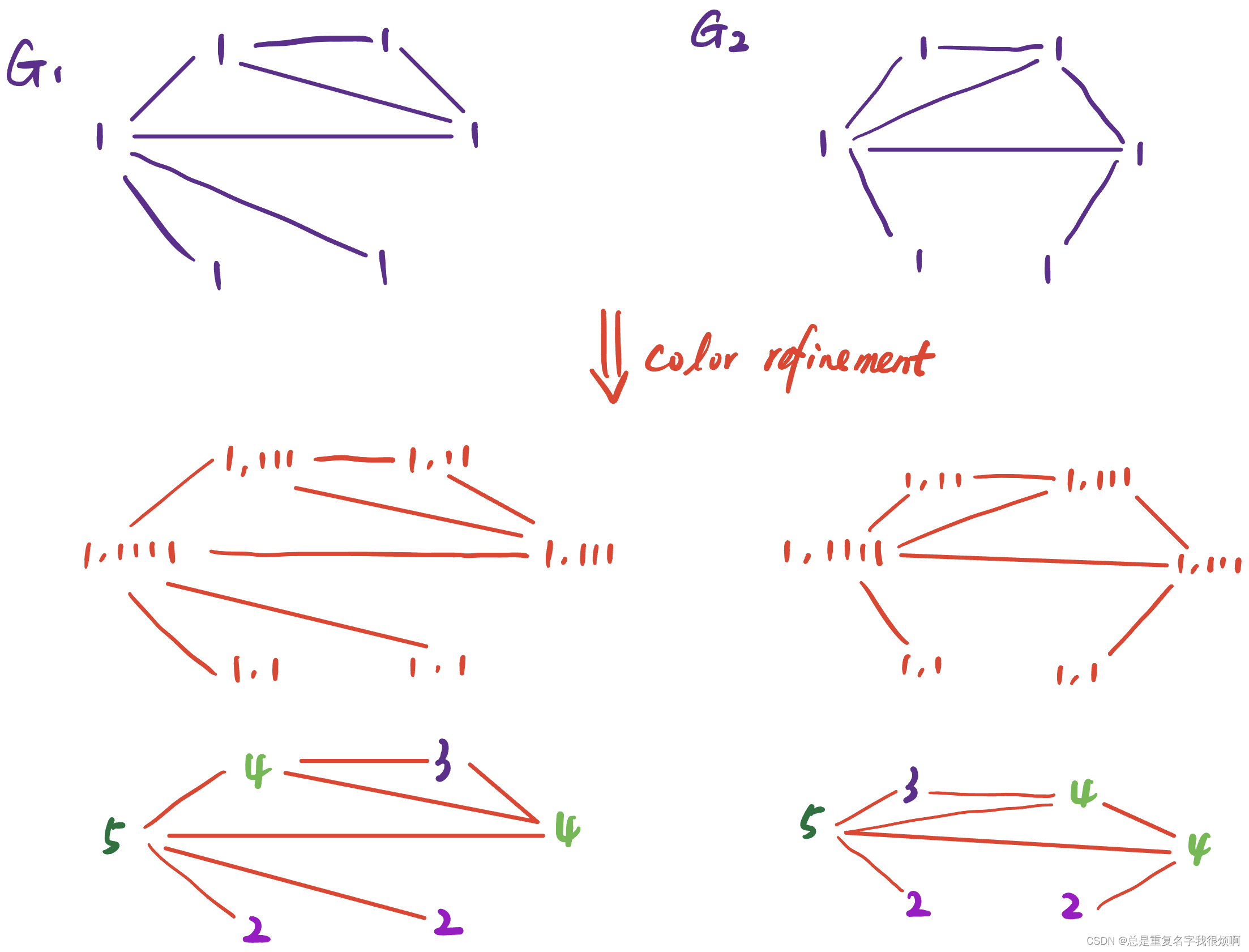
Assuming that the initial node is 1, then after the process of color refinement and hash map, it can become the bottom form. In this case, 1,1 corresponds to 2, 1,11 corresponds to 3, 1,111 corresponds to 4, and 1,1111 corresponds to 5. Of course, this picture can repeat this process and repeat it again, 2,4 corresponds to 6, 2,5 corresponds to 7, 3,44 corresponds to 8 and so on. Then you can turn the graph into a 13-dimensional vector.
For the graph on the left: [6,2,1,2,1,0,2,1,0,0,2,1,0]
For the graph on the right: [6,2,1,2,1, 1,1,0,1,1,1,0,1]

Graph Embedding Learning (Node Embedding) - Random Walk vs Matrix Factorization

This part follows the above, and it should also belong to the traditional graph machine learning part, but because its idea is very important, because whether it is graph machine learning or graph neural network, graph data needs to be mapped into a low-dimensional continuous dense vector, that is, node The embedding process, it can be said that the quality of the model is based on it. Therefore, it will be sorted out separately as a chapter.
The emergence of Node embedding means that artificial feature engineering has gradually withdrawn from the stage of history, and a graph representation and random walk methods have gradually entered people's field of vision. The nodes that appear together in the same random walk sequence are regarded as similar nodes, thus constructing a self-supervised learning scene similar to Word2Vec. Graph embedding methods based on random walks such as DeepWalk and Node2Vec are derived. Mathematically, random walk methods and matrix factorization are equivalent. Then discuss the method of embedding the whole graph, which can be realized by embedding vector aggregation of all nodes, introducing virtual nodes, anonymous random walk and other methods.

Before introducing this random walk method, it is recommended to intensively read the papers of DeepWalk and Node2Vec . And Node2Vec has similarities with Word2Vec to a certain extent. If you just want to learn graph network, you can directly read my article NLP from 0 , natural language into machine language-encoding chapter for a shallow understanding.