1. Features of graphs

The features that the graph points themselves have are called attribute features (such as: connection weight, node type, etc.), and attribute features are multimodal most of the time .

The connection relationship between a node and other nodes in the graph is called the connection feature (structural information)

The manually extracted and constructed features are called feature engineering . (Turn the graph into a vector) Feature engineering is generally constructed for the connection features of the graph

2. Feature engineering at the node level

In general, node-level connection features are divided into:

①The number of connections of the node

②The importance of nodes

③Aggregation coefficient of nodes (whether there is a connection between a node and its adjacent nodes)

④ Node subgraph information (how many artificially defined subgraphs around a node)

1. Number of node connections

If you want to find the number of node connections, you can directly sum according to a certain row/column; or multiply the adjacency matrix with a vector with a value of 1. However, the number of node connections does not consider the quality of connections, so the following three indicators are introduced to measure the quality of node connections.

2. Node importance

①Eigenvector Centrality

The importance of a node = the sum of the importance of its adjacent nodes , the formula is expressed as:

$c_v=\frac{1}{\lambda}\sum c_u$ where $\lambda$ only for normalization

Because it is a recursive algorithm, the actual calculation is converted to the problem of finding the eigenvector of the adjacency matrix A matrix

$\lambda c=Ac$ Where c is the eigenvector of the adjacency matrix A (composed of the importance of all nodes connected to the node); the adjacency matrix A is used to represent the connection attributes of these nodes; $\lambda$ that is, the importance of the target node.

②Betweenness Centrality

It is used to measure whether a node is at a traffic throat; the calculation method is: for all nodes in the connected domain except the required node , find out how many of the shortest distances must pass through the node. As shown below:

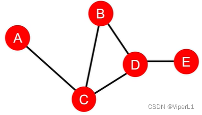
$c_A=c_B=c_E=0$ , while $c_C=3$ (path is: A- C -B, A- C -D, A- C -DE) $c_D=3$

3. Clustering Coefficient

The calculation method is: the number of connections between the surrounding nodes of the node/the number of connections between the node and the surrounding nodes, and the value range is [0,1]... (simple understanding is the number of triangles). See the example below for details:

The calculation results are: $e_v=\frac{6}{c_{4}^{2}}=1$ , $e_v=\frac{3}{c^2_4}=\frac{3}{6}=0.5$ , $e_v=\frac{0}{c^2_4}=0$

This triangular connection is called: ego- network

4.graphlet

The same number of nodes constitutes a non-isomorphic subgraph (similar to isomers). For example, 4 nodes can constitute 6 graphlets.

Extract the number of graphlets around a node to form a Graphlet Degree Vector (GDV), as shown in the following figure:

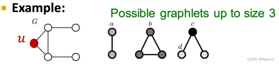
There are three possible subgraph forms for node u, and the types of subgraphs containing u nodes are listed respectively

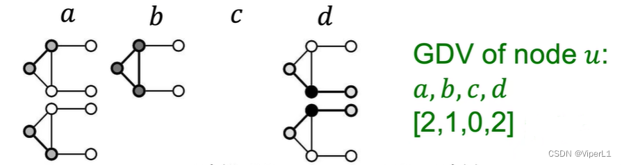
GDV can describe the local neighborhood topology information of node u .

3. Feature engineering at the connection level

Purpose: To complete unknown connections through known connections. There are two ways to obtain a D-dimensional vector:

① Directly extract the features of the connection

② Put together the D-dimensional vectors connecting the nodes at both ends (but this method will lose the connection information of the link itself)

The general method for connection prediction is:

① Get the connected D-dimensional vector

② Send the D-dimensional vector into machine learning for calculation and get the score $c(x,y)$

③ $c(x,y)$ Sort the scores and select the highest n new connections

④ Calculate the n predicted results and the real value

1. Connection features

Connection features are generally divided into: ① distance between nodes; ② local connection information of nodes; ③ connection information of nodes in the whole graph

①Shortest path length

That is, the number of nodes on the path with the least number of nodes between two points, but it is the same as the number of node connections, only the number and not the weight.

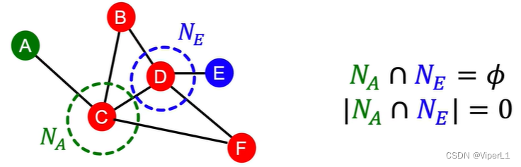
② Local connection information based on two nodes

The number of common adjacent nodes; intersection and union ratio, etc. However, if there is no local connection between the two nodes, the intersection ratio and the number of common adjacent nodes will be 0. For example, there is no local connection between A and E in the figure below.

③ Katz index

Indicates the number of paths of length k between node u and node v. Calculation method: use the power of the adjacency matrix to calculate, as follows:

$P_{uv}^{(2)}=\sum A_{ui}*P_{iv}^{(1)}=\sum_i A_{iv}=A_{uv}^2$

The actual meaning of this formula is: $A_{ui}$ =neighbor i who is 1 step away from u; $P_{iv}^{(1)}$ =whether i is 1 step away from v

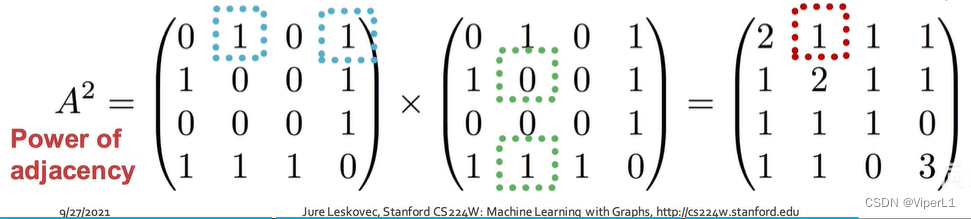
It can be known by mathematical induction that the matrix of length $l$ is $A_{uv}^l$ ( the element of row u and column v in the power of the matrix $A_{uv}$ $l$ )

The Katz coefficient formula can be simplified as:

$s=\sum \beta^iA^i=(I-\beta A)^{-1}-I$ where $\beta$ is the reduction factor, between 0 and 1; $I$ is the identity matrix.

4. Feature Engineering at the Full Image Level

The purpose is to extract the features of the entire image and turn it into a D-dimensional vector to reflect the structural characteristics of the entire image.

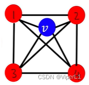
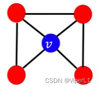
In fact, it is calculating the number of different features in the graph (think of the graph as an article, and the node as a word--Bag-of-Nodes)

But this method has a flaw, that is, it only looks at whether there is the i-th node and does not care about the connection structure. The D-dimensional vectors encoded in the two graphs in the figure below are consistent, both are [1 1 1 1 ]

Bag-of-Node-degrees can also be used, but the same only looks at the node dgree , not the node or the connection structure

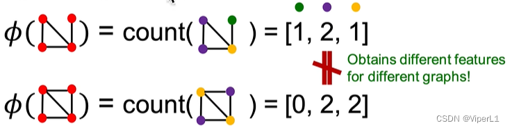
Bag-of-xxx can be extended to any of the features mentioned above . For example, the graphlets of the whole graph are used as the application scenario. Compared with the graphlets at the node level, there are the following differences: ① isolated nodes can exist ; ② the counting object is the whole graph , rather than specific node neighborhoods.

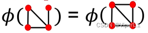
The Graphlet Kernel (a scalar quantity) can be obtained by multiplying the graphlets of the two graphs . This index can reflect whether the two graphs are similar/matching. The formula is recorded as:

$K(G,{G}')=f_g^Tf{G}'$

If the sizes of the two images are inconsistent, they need to be normalized

But this approach consumes a lot of computing power . Therefore, the Weisfeiler-Lehman Kernel algorithm is generally used , and the idea of color refinement ( Color refinement ) is adopted . The specific method is as follows:

① Initialize the graph with a code

②Adjust the code according to the number of connections of specific nodes

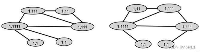
③Replace different codes with different colors (Hash)

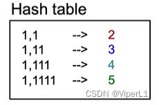
The above steps can be repeated, and the last two nodes with the same structure will always have the same color

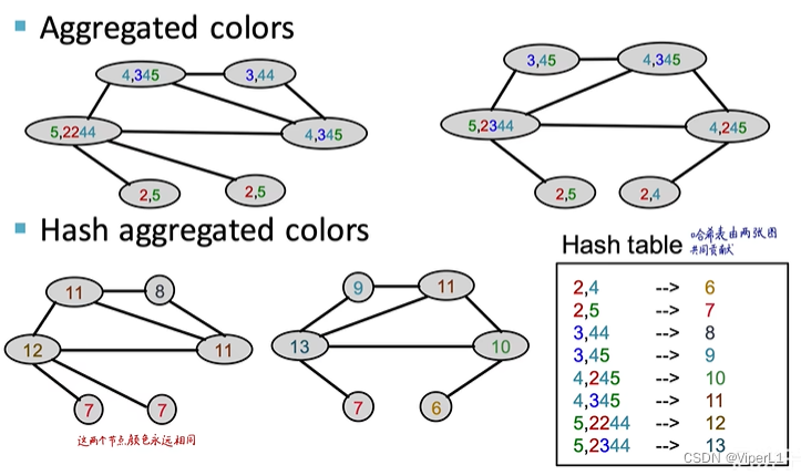
This turns each graph into a lower-dimensional vector. The Weisfeiler-Lehman kernel can be obtained by taking the inner product of the vectors of these two graphs

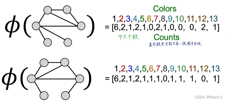
The above operations can be recorded as: $c^{(k+1)}(v)=HASH(\{c^{(k)}(v),\{c^{(k)}(u)\}_{u \in N(v)}\})$ , k means that the above encoding process has carried out k steps, and means that k jump connections in the figure have been captured

[Graph Neural Network] Graph Feature Engineering