Tensorflow2.0之绘图：分类问题的准确率、精确率、召回率、ROC曲线以及曲线下面积

准确率、精确率、召回率、ROC曲线的定义

阳性与阴性
准确率
精确率与召回率
ROC 和曲线下面积

用Tensorflow2.0绘制相关曲线

建模时设置METRICS

METRICS = [
      keras.metrics.TruePositives(name='tp'),
      keras.metrics.FalsePositives(name='fp'),
      keras.metrics.TrueNegatives(name='tn'),
      keras.metrics.FalseNegatives(name='fn'), 
      keras.metrics.BinaryAccuracy(name='accuracy'),
      keras.metrics.Precision(name='precision'),
      keras.metrics.Recall(name='recall'),
      keras.metrics.AUC(name='auc'),
]

model = keras.Sequential([
  keras.layers.Dense(16, activation='relu', input_shape=(train_features.shape[-1],)),
  keras.layers.Dropout(0.5),
  keras.layers.Dense(1, activation='sigmoid')
])

model.compile(
  optimizer=keras.optimizers.Adam(lr=1e-3),
  loss=keras.losses.BinaryCrossentropy(),
  metrics=METRICS)
  
history = model.fit(
    train_features,
    train_labels,
    batch_size=BATCH_SIZE,
    epochs=EPOCHS,
    validation_data=(val_features, val_labels))

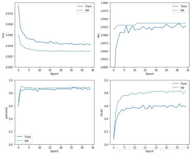
定义损失曲线、AUC曲线、精确率曲线以及召回率曲线函数

def plot_metrics(history):
    metrics =  ['loss', 'auc', 'precision', 'recall']
    for n, metric in enumerate(metrics):
        name = metric
        plt.subplot(2,2,n+1)
        plt.plot(history.epoch,  history.history[metric], color=colors[0], label='Train')
        plt.plot(history.epoch, history.history['val_'+metric],
                 color=colors[0], linestyle="--", label='Val')
        plt.xlabel('Epoch')
        plt.ylabel(name)
        if metric == 'loss':
            plt.ylim([0, plt.ylim()[1]])
        elif metric == 'auc':
            plt.ylim([0.8,1])
        else:
            plt.ylim([0,1])

        plt.legend()
plot_metrics(baseline_history)

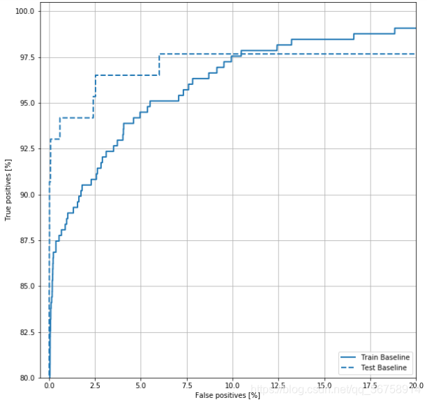
定义ROC曲线函数

def plot_roc(name, labels, predictions, **kwargs):
    fp, tp, _ = sklearn.metrics.roc_curve(labels, predictions)

    plt.plot(100*fp, 100*tp, label=name, linewidth=2, **kwargs)
    plt.xlabel('False positives [%]')
    plt.ylabel('True positives [%]')
    plt.xlim([-0.5,20])
    plt.ylim([80,100.5])
    plt.grid(True)
    ax = plt.gca()
    ax.set_aspect('equal')

预测训练集和测试集

train_predictions = model.predict(train_features, batch_size=BATCH_SIZE)
test_predictions = model.predict(test_features, batch_size=BATCH_SIZE)

ROC曲线

plot_roc("Train Baseline", train_labels, train_predictions, color=colors[0])
plot_roc("Test Baseline", test_labels, test_predictions, color=colors[0], linestyle='--')
plt.legend(loc='lower right')

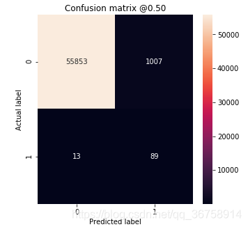
定义混淆矩阵函数

def plot_cm(labels, predictions, p=0.5):
    cm = confusion_matrix(labels, predictions > p)
    plt.figure(figsize=(5,5))
    sns.heatmap(cm, annot=True, fmt="d")
    plt.title('Confusion matrix @{:.2f}'.format(p))
    plt.ylabel('Actual label')
    plt.xlabel('Predicted label')

绘制混淆矩阵

plot_cm(test_labels, test_predictions)