睿智的目标检测17——Keras搭建Retinanet目标检测平台

学习前言

一起来看看Retinanet的keras实现吧，顺便训练一下自己的数据。

什么是Retinanet目标检测算法

Retinanet是在何凯明大神提出Focal loss同时提出的一种新的目标检测方案，来验证Focal Loss的有效性。

One-Stage目标检测方法常常使用先验框提高预测性能，一张图像可能生成成千上万的候选框，但是其中只有很少一部分是包含目标的的，有目标的就是正样本，没有目标的就是负样本。这种情况造成了One-Stage目标检测方法的正负样本不平衡，也使得One-Stage目标检测方法的检测效果比不上Two-Stage目标检测方法。

Focal Loss是一种新的用于平衡One-Stage目标检测方法正负样本的Loss方案。

Retinane的结构非常简单，但是其存在非常多的先验框，以输入600x600x3的图片为例，就存在着67995个先验框，这些先验框里面大多包含的是背景，存在非常多的负样本。以Focal Loss训练的Retinanet可以有效的平衡正负样本，实现有效的训练。

源码下载

https://github.com/bubbliiiing/retinanet-keras
喜欢的可以点个star噢。

Retinanet实现思路

一、预测部分

1、主干网络介绍

Retinanet采用的主干网络是Resnet网络，关于Resnet的介绍大家可以看我的另外一篇博客https://blog.csdn.net/weixin_44791964/article/details/102790260。

本例子假设输入的图片大小为600x600x3。

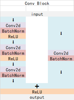
ResNet50有两个基本的块，分别名为Conv Block和Identity Block，其中Conv Block输入和输出的维度是不一样的，所以不能连续串联，它的作用是改变网络的维度；Identity Block输入维度和输出维度相同，可以串联，用于加深网络的。
Conv Block的结构如下：

Identity Block的结构如下：

这两个都是残差网络结构。

扫描二维码关注公众号，回复： 9576914 查看本文章

当输入的图片为600x600x3的时候，shape变化与总的网络结构如下：

我们取出长宽压缩了三次、四次、五次的结果来进行网络金字塔结构的构造。

实现代码：

#-------------------------------------------------------------#
#   ResNet50的网络部分
#-------------------------------------------------------------#
from __future__ import print_function

import numpy as np
from keras import layers

from keras.layers import Input
from keras.layers import Dense,Conv2D,MaxPooling2D,ZeroPadding2D,AveragePooling2D
from keras.layers import Activation,BatchNormalization,Flatten
from keras.models import Model

from keras.preprocessing import image
import keras.backend as K
from keras.utils.data_utils import get_file
from keras.applications.imagenet_utils import decode_predictions
from keras.applications.imagenet_utils import preprocess_input


def identity_block(input_tensor, kernel_size, filters, stage, block):

    filters1, filters2, filters3 = filters

    conv_name_base = 'res' + str(stage) + block + '_branch'
    bn_name_base = 'bn' + str(stage) + block + '_branch'

    x = Conv2D(filters1, (1, 1), name=conv_name_base + '2a',use_bias=False)(input_tensor)
    x = BatchNormalization(name=bn_name_base + '2a')(x)
    x = Activation('relu')(x)

    x = Conv2D(filters2, kernel_size,padding='same', name=conv_name_base + '2b',use_bias=False)(x)

    x = BatchNormalization(name=bn_name_base + '2b')(x)
    x = Activation('relu')(x)

    x = Conv2D(filters3, (1, 1), name=conv_name_base + '2c',use_bias=False)(x)
    x = BatchNormalization(name=bn_name_base + '2c')(x)

    x = layers.add([x, input_tensor])
    x = Activation('relu')(x)
    return x


def conv_block(input_tensor, kernel_size, filters, stage, block, strides=(2, 2)):

    filters1, filters2, filters3 = filters

    conv_name_base = 'res' + str(stage) + block + '_branch'
    bn_name_base = 'bn' + str(stage) + block + '_branch'

    x = Conv2D(filters1, (1, 1), strides=strides,
               name=conv_name_base + '2a',use_bias=False)(input_tensor)
    x = BatchNormalization(name=bn_name_base + '2a')(x)
    x = Activation('relu')(x)

    x = Conv2D(filters2, kernel_size, padding='same',
               name=conv_name_base + '2b',use_bias=False)(x)
    x = BatchNormalization(name=bn_name_base + '2b')(x)
    x = Activation('relu')(x)

    x = Conv2D(filters3, (1, 1), name=conv_name_base + '2c',use_bias=False)(x)
    x = BatchNormalization(name=bn_name_base + '2c')(x)

    shortcut = Conv2D(filters3, (1, 1), strides=strides,
                      name=conv_name_base + '1',use_bias=False)(input_tensor)
    shortcut = BatchNormalization(name=bn_name_base + '1')(shortcut)

    x = layers.add([x, shortcut])
    x = Activation('relu')(x)
    return x


def ResNet50(inputs):

    img_input = inputs
    x = ZeroPadding2D((3, 3))(img_input)

    x = Conv2D(64, (7, 7), strides=(2, 2), name='conv1',use_bias=False)(x)
    x = BatchNormalization(name='bn_conv1')(x)
    x = Activation('relu')(x)
    x = MaxPooling2D((3, 3), strides=(2, 2), padding="same")(x)

    x = conv_block(x, 3, [64, 64, 256], stage=2, block='a', strides=(1, 1))
    x = identity_block(x, 3, [64, 64, 256], stage=2, block='b')
    x = identity_block(x, 3, [64, 64, 256], stage=2, block='c')
    y0 = x
    x = conv_block(x, 3, [128, 128, 512], stage=3, block='a')
    x = identity_block(x, 3, [128, 128, 512], stage=3, block='b')
    x = identity_block(x, 3, [128, 128, 512], stage=3, block='c')
    x = identity_block(x, 3, [128, 128, 512], stage=3, block='d')
    y1 = x
    x = conv_block(x, 3, [256, 256, 1024], stage=4, block='a')
    x = identity_block(x, 3, [256, 256, 1024], stage=4, block='b')
    x = identity_block(x, 3, [256, 256, 1024], stage=4, block='c')
    x = identity_block(x, 3, [256, 256, 1024], stage=4, block='d')
    x = identity_block(x, 3, [256, 256, 1024], stage=4, block='e')
    x = identity_block(x, 3, [256, 256, 1024], stage=4, block='f')
    y2 = x
    x = conv_block(x, 3, [512, 512, 2048], stage=5, block='a')
    x = identity_block(x, 3, [512, 512, 2048], stage=5, block='b')
    x = identity_block(x, 3, [512, 512, 2048], stage=5, block='c')
    y3 = x
    model = Model(img_input, [y0,y1,y2,y3], name='resnet50')

    return model

2、从特征获取预测结果

由抽象的结构图可知，获得到的特征还需要经过图像金字塔的处理，这样的结构可以融合多尺度的特征，实现更有效的预测。

图像金字塔的具体结构如下：

通过图像金字塔我们可以获得五个有效的特征层，分别是P3、P4、P5、P6、P7，
为了和普通特征层区分，我们称之为有效特征层，将这五个有效的特征层传输过class+box subnets就可以获得预测结果了。

class subnet采用4次256通道的卷积和1次num_priors x num_classes的卷积，num_priors指的是该特征层所拥有的先验框数量，num_classes指的是网络一共对多少类的目标进行检测。

box subnet采用4次256通道的卷积和1次num_priors x 4的卷积，num_priors指的是该特征层所拥有的先验框数量，4指的是先验框的调整情况。

需要注意的是，每个特征层所用的class subnet是同一个class subnet；每个特征层所用的box subnet是同一个box subnet。

其中：
num_priors x 4的卷积 用于预测 该特征层上 每一个网格点上 每一个先验框的变化情况。（为什么说是变化情况呢，这是因为ssd的预测结果需要结合先验框获得预测框，预测结果就是先验框的变化情况。）

num_priors x num_classes的卷积 用于预测 该特征层上 每一个网格点上 每一个预测框对应的种类。

实现代码为：

import keras
import keras.layers

from nets.resnet import ResNet50
from utils.anchors import AnchorParameters
from utils.utils import PriorProbability
from nets import layers

def make_last_layer_loc(num_classes,num_anchors,pyramid_feature_size=256):

    inputs = keras.layers.Input(shape=(None, None, pyramid_feature_size)) 

    options = {
        'kernel_size'        : 3,
        'strides'            : 1,
        'padding'            : 'same',
        'kernel_initializer' : keras.initializers.normal(mean=0.0, stddev=0.01, seed=None),
        'bias_initializer'   : 'zeros'
    }
    outputs = inputs
    for i in range(4):
        outputs = keras.layers.Conv2D(filters=256,activation='relu',name='pyramid_regression_{}'.format(i),**options)(outputs)

    outputs = keras.layers.Conv2D(num_anchors * 4, name='pyramid_regression', **options)(outputs)
    
    regression = keras.layers.Reshape((-1, 4), name='pyramid_regression_reshape')(outputs)
    
    regression_model = keras.models.Model(inputs=inputs, outputs=regression, name="regression_submodel")
    return regression_model


def make_last_layer_cls(num_classes,num_anchors,pyramid_feature_size=256):
    
    inputs = keras.layers.Input(shape=(None, None, pyramid_feature_size))

    options = {
        'kernel_size' : 3,
        'strides'     : 1,
        'padding'     : 'same',
    }
    classification = [] 
    outputs = inputs

    for i in range(4):
        outputs = keras.layers.Conv2D(
            filters=256,
            activation='relu',
            name='pyramid_classification_{}'.format(i),
            kernel_initializer=keras.initializers.normal(mean=0.0, stddev=0.01, seed=None),
            bias_initializer='zeros',
            **options
        )(outputs)

    outputs = keras.layers.Conv2D(filters=num_classes * num_anchors,
        kernel_initializer=keras.initializers.normal(mean=0.0, stddev=0.01, seed=None),
        bias_initializer=PriorProbability(probability=0.01),
        name='pyramid_classification'.format(),
        **options
    )(outputs)

    outputs = keras.layers.Reshape((-1, num_classes), name='pyramid_classification_reshape')(outputs)
    classification = keras.layers.Activation('sigmoid', name='pyramid_classification_sigmoid')(outputs)

    classification_model = keras.models.Model(inputs=inputs, outputs=classification, name="classification_submodel")
    return classification_model


def resnet_retinanet(num_classes, inputs=None, num_anchors=None, submodels=None, name='retinanet'):
    if inputs==None:
        inputs = keras.layers.Input(shape=(600, 600, 3))
    else:
        inputs = inputs
    resnet = ResNet50(inputs)
    
    if num_anchors is None:
        num_anchors = AnchorParameters.default.num_anchors()

    C3, C4, C5 = resnet.outputs[1:]

    P5           = keras.layers.Conv2D(256, kernel_size=1, strides=1, padding='same', name='C5_reduced')(C5)
    P5_upsampled = layers.UpsampleLike(name='P5_upsampled')([P5, C4])
    P5           = keras.layers.Conv2D(256, kernel_size=3, strides=1, padding='same', name='P5')(P5)
    
    P4           = keras.layers.Conv2D(256, kernel_size=1, strides=1, padding='same', name='C4_reduced')(C4)
    P4           = keras.layers.Add(name='P4_merged')([P5_upsampled, P4])
    P4_upsampled = layers.UpsampleLike(name='P4_upsampled')([P4, C3])
    P4           = keras.layers.Conv2D(256, kernel_size=3, strides=1, padding='same', name='P4')(P4)

    P3 = keras.layers.Conv2D(256, kernel_size=1, strides=1, padding='same', name='C3_reduced')(C3)
    P3 = keras.layers.Add(name='P3_merged')([P4_upsampled, P3])
    P3 = keras.layers.Conv2D(256, kernel_size=3, strides=1, padding='same', name='P3')(P3)

    P6 = keras.layers.Conv2D(256, kernel_size=3, strides=2, padding='same', name='P6')(C5)

    P7 = keras.layers.Activation('relu', name='C6_relu')(P6)
    P7 = keras.layers.Conv2D(256, kernel_size=3, strides=2, padding='same', name='P7')(P7)

    features =  [P3, P4, P5, P6, P7]

    regression_model = make_last_layer_loc(num_classes,num_anchors)
    classification_model = make_last_layer_cls(num_classes,num_anchors)

    regressions = []
    classifications = []
    for feature in features:
        regression = regression_model(feature)
        classification = classification_model(feature)
        regressions.append(regression)
        classifications.append(classification)

    regressions = keras.layers.Concatenate(axis=1, name="regression")(regressions)
    classifications = keras.layers.Concatenate(axis=1, name="classification")(classifications)
    pyramids = [regressions,classifications]

    model = keras.models.Model(inputs=inputs, outputs=pyramids, name=name)

    return model

3、预测结果的解码

我们通过对每一个特征层的处理，可以获得三个内容，分别是：

num_priors x 4的卷积 用于预测 该特征层上 每一个网格点上 每一个先验框的变化情况。**

num_priors x num_classes的卷积 用于预测 该特征层上 每一个网格点上 每一个预测框对应的种类。

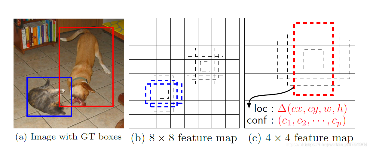
每一个有效特征层对应的先验框对应着该特征层上 每一个网格点上 预先设定好的9个框。

我们利用 num_priors x 4的卷积 与 每一个有效特征层对应的先验框 获得框的真实位置。

每一个有效特征层对应的先验框就是，如图所示的作用：
每一个有效特征层将整个图片分成与其长宽对应的网格，如P3的特征层就是将整个图像分成75x75个网格；然后从每个网格中心建立9个先验框，一共75x75x9个，50625个先验框。

先验框虽然可以代表一定的框的位置信息与框的大小信息，但是其是有限的，无法表示任意情况，因此还需要调整，Retinanet利用4次256通道的卷积+num_priors x 4的卷积的结果对先验框进行调整。

num_priors x 4中的num_priors表示了这个网格点所包含的先验框数量，其中的4表示了框的左上角xy轴，右下角xy的调整情况。

Retinanet解码过程就是将对应的先验框的左上角和右下角进行位置的调整，调整完的结果就是预测框的位置了。

当然得到最终的预测结构后还要进行得分排序与非极大抑制筛选这一部分基本上是所有目标检测通用的部分。
1、取出每一类得分大于confidence_threshold的框和得分。
2、利用框的位置和得分进行非极大抑制。
实现代码如下：

def decode_boxes(self, mbox_loc, mbox_priorbox):
    # 获得先验框的宽与高
    prior_width = mbox_priorbox[:, 2] - mbox_priorbox[:, 0]
    prior_height = mbox_priorbox[:, 3] - mbox_priorbox[:, 1]

    # 获取真实框的左上角与右下角
    decode_bbox_xmin = mbox_loc[:,0]*prior_width*0.2 + mbox_priorbox[:, 0]
    decode_bbox_ymin = mbox_loc[:,1]*prior_height*0.2 + mbox_priorbox[:, 1]
    decode_bbox_xmax = mbox_loc[:,2]*prior_width*0.2 + mbox_priorbox[:, 2]
    decode_bbox_ymax = mbox_loc[:,3]*prior_height*0.2 + mbox_priorbox[:, 3]

    # 真实框的左上角与右下角进行堆叠
    decode_bbox = np.concatenate((decode_bbox_xmin[:, None],
                                    decode_bbox_ymin[:, None],
                                    decode_bbox_xmax[:, None],
                                    decode_bbox_ymax[:, None]), axis=-1)
    # 防止超出0与1
    decode_bbox = np.minimum(np.maximum(decode_bbox, 0.0), 1.0)
    return decode_bbox

def detection_out(self, predictions, mbox_priorbox, keep_top_k=200,
                    confidence_threshold=0.4):
    
    # 网络预测的结果
    mbox_loc = predictions[0]
    # 先验框
    mbox_priorbox = mbox_priorbox
    # 置信度
    mbox_conf = predictions[1]
    results = []
    # 对每一个图片进行处理
    for i in range(len(mbox_loc)):
        results.append([])
        decode_bbox = self.decode_boxes(mbox_loc[i], mbox_priorbox)
        for c in range(self.num_classes):
            c_confs = mbox_conf[i, :, c]
            c_confs_m = c_confs > confidence_threshold
            if len(c_confs[c_confs_m]) > 0:
                # 取出得分高于confidence_threshold的框
                boxes_to_process = decode_bbox[c_confs_m]
                confs_to_process = c_confs[c_confs_m]
                # 进行iou的非极大抑制
                feed_dict = {self.boxes: boxes_to_process,
                                self.scores: confs_to_process}
                idx = self.sess.run(self.nms, feed_dict=feed_dict)
                # 取出在非极大抑制中效果较好的内容
                good_boxes = boxes_to_process[idx]
                confs = confs_to_process[idx][:, None]
                # 将label、置信度、框的位置进行堆叠。
                labels = c * np.ones((len(idx), 1))
                c_pred = np.concatenate((labels, confs, good_boxes),
                                        axis=1)
                # 添加进result里
                results[-1].extend(c_pred)

        if len(results[-1]) > 0:
            # 按照置信度进行排序
            results[-1] = np.array(results[-1])
            argsort = np.argsort(results[-1][:, 1])[::-1]
            results[-1] = results[-1][argsort]
            # 选出置信度最大的keep_top_k个
            results[-1] = results[-1][:keep_top_k]
    # 获得，在所有预测结果里面，置信度比较高的框
    # 还有，利用先验框和Retinanet的预测结果，处理获得了真实框（预测框）的位置
    return results

4、在原图上进行绘制

通过第三步，我们可以获得预测框在原图上的位置，而且这些预测框都是经过筛选的。这些筛选后的框可以直接绘制在图片上，就可以获得结果了。

二、训练部分

1、真实框的处理

从预测部分我们知道，每个特征层的预测结果，num_priors x 4的卷积 用于预测 该特征层上 每一个网格点上 每一个先验框的变化情况。

也就是说，我们直接利用retinanet网络预测到的结果，并不是预测框在图片上的真实位置，需要解码才能得到真实位置。

而在训练的时候，我们需要计算loss函数，这个loss函数是相对于Retinanet网络的预测结果的。我们需要把图片输入到当前的Retinanet网络中，得到预测结果；同时还需要把真实框的信息，进行编码，这个编码是把真实框的位置信息格式转化为Retinanet预测结果的格式信息。

也就是，我们需要找到 每一张用于训练的图片的每一个真实框对应的先验框，并求出如果想要得到这样一个真实框，我们的预测结果应该是怎么样的。

从预测结果获得真实框的过程被称作解码，而从真实框获得预测结果的过程就是编码的过程。

因此我们只需要将解码过程逆过来就是编码过程了。

实现代码如下：

def encode_box(self, box, return_iou=True):
    iou = self.iou(box)
    encoded_box = np.zeros((self.num_priors, 4 + return_iou))

    # 找到每一个真实框，重合程度较高的先验框
    assign_mask = iou > self.overlap_threshold
    if not assign_mask.any():
        assign_mask[iou.argmax()] = True
    if return_iou:
        encoded_box[:, -1][assign_mask] = iou[assign_mask]
    
    # 找到对应的先验框
    assigned_priors = self.priors[assign_mask]
    # 逆向编码，将真实框转化为Retinanet预测结果的格式
    assigned_priors_w = (assigned_priors[:, 2] -
                            assigned_priors[:, 0])

    assigned_priors_h = (assigned_priors[:, 3] -
                            assigned_priors[:, 1])
                            
    encoded_box[:,0][assign_mask] = (box[0] - assigned_priors[:, 0])/assigned_priors_w/0.2
    encoded_box[:,1][assign_mask] = (box[1] - assigned_priors[:, 1])/assigned_priors_h/0.2
    encoded_box[:,2][assign_mask] = (box[2] - assigned_priors[:, 2])/assigned_priors_w/0.2
    encoded_box[:,3][assign_mask] = (box[3] - assigned_priors[:, 3])/assigned_priors_h/0.2

    return encoded_box.ravel()

利用上述代码我们可以获得，真实框对应的所有的iou较大先验框，并计算了真实框对应的所有iou较大的先验框应该有的预测结果。

但是由于原始图片中可能存在多个真实框，可能同一个先验框会与多个真实框重合度较高，我们只取其中与真实框重合度最高的就可以了。

因此我们还要经过一次筛选，将上述代码获得的真实框对应的所有的iou较大先验框的预测结果中，iou最大的那个真实框筛选出来。

通过assign_boxes我们就获得了，输入进来的这张图片，应该有的预测结果是什么样子的。

实现代码如下：

def assign_boxes(self, boxes):
    assignment = np.zeros((self.num_priors, 4 + 1 + self.num_classes + 1))
    assignment[:, 4] = 0.0
    assignment[:, -1] = 0.0
    if len(boxes) == 0:
        return assignment
    # 对每一个真实框都进行iou计算
    ingored_boxes = np.apply_along_axis(self.ignore_box, 1, boxes[:, :4])
    # 取重合程度最大的先验框，并且获取这个先验框的index
    ingored_boxes = ingored_boxes.reshape(-1, self.num_priors, 1)
    # (num_priors)
    ignore_iou = ingored_boxes[:, :, 0].max(axis=0)
    # (num_priors)
    ignore_iou_mask = ignore_iou > 0

    assignment[:, 4][ignore_iou_mask] = -1
    assignment[:, -1][ignore_iou_mask] = -1

    # (n, num_priors, 5)
    encoded_boxes = np.apply_along_axis(self.encode_box, 1, boxes[:, :4])
    # 每一个真实框的编码后的值，和iou
    # (n, num_priors)
    encoded_boxes = encoded_boxes.reshape(-1, self.num_priors, 5)

    # 取重合程度最大的先验框，并且获取这个先验框的index
    # (num_priors)
    best_iou = encoded_boxes[:, :, -1].max(axis=0)
    # (num_priors)
    best_iou_idx = encoded_boxes[:, :, -1].argmax(axis=0)
    # (num_priors)
    best_iou_mask = best_iou > 0
    # 某个先验框它属于哪个真实框
    best_iou_idx = best_iou_idx[best_iou_mask]

    assign_num = len(best_iou_idx)
    # 保留重合程度最大的先验框的应该有的预测结果
    # 哪些先验框存在真实框
    encoded_boxes = encoded_boxes[:, best_iou_mask, :]

    assignment[:, :4][best_iou_mask] = encoded_boxes[best_iou_idx,np.arange(assign_num),:4]
    # 4代表为背景的概率，为0
    assignment[:, 4][best_iou_mask] = 1
    assignment[:, 5:-1][best_iou_mask] = boxes[best_iou_idx, 4:]
    assignment[:, -1][best_iou_mask] = 1
    # 通过assign_boxes我们就获得了，输入进来的这张图片，应该有的预测结果是什么样子的

    return assignment

focal会忽略一些重合度相对较高但是不是非常高的先验框，一般将重合度在0.4-0.5之间的先验框进行忽略。
实现代码如下：

def ignore_box(self, box):
    iou = self.iou(box)
    ignored_box = np.zeros((self.num_priors, 1))

    # 找到每一个真实框，重合程度较高的先验框
    assign_mask = (iou > self.ignore_threshold)&(iou<self.overlap_threshold)

    if not assign_mask.any():
        assign_mask[iou.argmax()] = True
        
    ignored_box[:, 0][assign_mask] = iou[assign_mask]
    return ignored_box.ravel()

2、利用处理完的真实框与对应图片的预测结果计算loss

loss的计算分为两个部分：
1、Smooth Loss：获取所有正标签的框的预测结果的回归loss。
2、Focal Loss：获取所有未被忽略的种类的预测结果的交叉熵loss。

由于在Retinanet的训练过程中，正负样本极其不平衡，即 存在对应真实框的先验框可能只有若干个，但是不存在对应真实框的负样本却有上万个，这就会导致负样本的loss值极大，因此引入了Focal Loss进行正负样本的平衡，关于Focal Loss的介绍可以看这个博客。
https://blog.csdn.net/weixin_44791964/article/details/102853782

实现代码如下：

def focal(alpha=0.25, gamma=2.0):
    def _focal(y_true, y_pred):
        # y_true [batch_size, num_anchor, num_classes+1]
        # y_pred [batch_size, num_anchor, num_classes]
        labels         = y_true[:, :, :-1]
        anchor_state   = y_true[:, :, -1]  # -1 是需要忽略的, 0 是背景, 1 是存在目标
        classification = y_pred

        # 找出存在目标的先验框
        indices_for_object        = tf.where(keras.backend.equal(anchor_state, 1))
        labels_for_object         = tf.gather_nd(labels, indices_for_object)
        classification_for_object = tf.gather_nd(classification, indices_for_object)

        # 计算每一个先验框应该有的权重
        alpha_factor_for_object = keras.backend.ones_like(labels_for_object) * alpha
        focal_weight_for_object = 1 - classification_for_object
        focal_weight_for_object = alpha_factor_for_object * focal_weight_for_object ** gamma

        # 将权重乘上所求得的交叉熵
        cls_loss_for_object = focal_weight_for_object * keras.backend.binary_crossentropy(labels_for_object, classification_for_object)

        # 找出实际上为背景的先验框
        indices_for_back        = tf.where(keras.backend.equal(anchor_state, 0))
        labels_for_back         = tf.gather_nd(labels, indices_for_back)
        classification_for_back = tf.gather_nd(classification, indices_for_back)

        # 计算每一个先验框应该有的权重
        alpha_factor_for_back = keras.backend.ones_like(labels_for_back) * (1-alpha)
        focal_weight_for_back = classification_for_back
        focal_weight_for_back = alpha_factor_for_back * focal_weight_for_back ** gamma

        # 将权重乘上所求得的交叉熵
        cls_loss_for_back = focal_weight_for_back * keras.backend.binary_crossentropy(labels_for_back, classification_for_back)

        # 标准化，实际上是正样本的数量
        normalizer = tf.where(keras.backend.equal(anchor_state, 1))
        normalizer = keras.backend.cast(keras.backend.shape(normalizer)[0], keras.backend.floatx())
        normalizer = keras.backend.maximum(keras.backend.cast_to_floatx(1.0), normalizer)

        # 将所获得的loss除上正样本的数量
        cls_loss_for_object = keras.backend.sum(cls_loss_for_object)/normalizer
        cls_loss_for_back = keras.backend.sum(cls_loss_for_back)/normalizer

        # 总的loss
        loss = cls_loss_for_object + cls_loss_for_back

        # loss = tf.Print(loss, [loss, cls_loss_for_object, cls_loss_for_back], message='\nloss: ')
    
        return loss
    return _focal
    
def smooth_l1(sigma=1.0):
    sigma_squared = sigma ** 2

    def _smooth_l1(y_true, y_pred):
        # y_true [batch_size, num_anchor, 4+1]
        # y_pred [batch_size, num_anchor, 4]
        regression        = y_pred
        regression_target = y_true[:, :, :-1]
        anchor_state      = y_true[:, :, -1]

        # 找到正样本
        indices           = tf.where(keras.backend.equal(anchor_state, 1))
        regression        = tf.gather_nd(regression, indices)
        regression_target = tf.gather_nd(regression_target, indices)

        # 计算 smooth L1 loss
        # f(x) = 0.5 * (sigma * x)^2          if |x| < 1 / sigma / sigma
        #        |x| - 0.5 / sigma / sigma    otherwise
        regression_diff = regression - regression_target
        regression_diff = keras.backend.abs(regression_diff)
        regression_loss = backend.where(
            keras.backend.less(regression_diff, 1.0 / sigma_squared),
            0.5 * sigma_squared * keras.backend.pow(regression_diff, 2),
            regression_diff - 0.5 / sigma_squared
        )

        normalizer = keras.backend.maximum(1, keras.backend.shape(indices)[0])
        normalizer = keras.backend.cast(normalizer, dtype=keras.backend.floatx())
        loss = keras.backend.sum(regression_loss) / normalizer

        return loss

    return _smooth_l1

训练自己的Retinanet模型

Retinanet整体的文件夹构架如下：

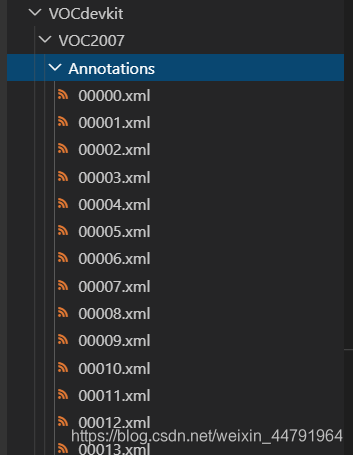
本文使用VOC格式进行训练。
训练前将标签文件放在VOCdevkit文件夹下的VOC2007文件夹下的Annotation中。

训练前将图片文件放在VOCdevkit文件夹下的VOC2007文件夹下的JPEGImages中。

在训练前利用voc2retinanet.py文件生成对应的txt。

再运行根目录下的voc_annotation.py，运行前需要将classes改成你自己的classes。

classes = ["aeroplane", "bicycle", "bird", "boat", "bottle", "bus", "car", "cat", "chair", "cow", "diningtable", "dog", "horse", "motorbike", "person", "pottedplant", "sheep", "sofa", "train", "tvmonitor"]

就会生成对应的2007_train.txt，每一行对应其图片位置及其真实框的位置。

在训练前需要修改model_data里面的voc_classes.txt文件，需要将classes改成你自己的classes。

运行train.py即可开始训练。