睿智的目标检测54——Tensorflow2 搭建YoloX目标检测平台
学习前言
旷视新提出了YoloX,感觉蛮有意思,复现一下哈哈。

源码下载
https://github.com/bubbliiiing/yolox-tf2
喜欢的可以点个star噢。
YoloX改进的部分(不完全)
1、主干部分:使用了Focus网络结构,这个结构是在YoloV5里面使用到比较有趣的网络结构,具体操作是在一张图片中每隔一个像素拿到一个值,这个时候获得了四个独立的特征层,然后将四个独立的特征层进行堆叠,此时宽高信息就集中到了通道信息,输入通道扩充了四倍。
2、分类回归层:Decoupled Head,以前版本的Yolo所用的解耦头是一起的,也就是分类和回归在一个1X1卷积里实现,YoloX认为这给网络的识别带来了不利影响。在YoloX中,Yolo Head被分为了两部分,分别实现,最后预测的时候才整合在一起。
3、数据增强:Mosaic数据增强、Mosaic利用了四张图片进行拼接实现数据中增强,根据论文所说其拥有一个巨大的优点是丰富检测物体的背景!且在BN计算的时候一下子会计算四张图片的数据!
4、Anchor Free:不使用先验框。
5、SimOTA :为不同大小的目标动态匹配正样本。
以上并非全部的改进部分,还存在一些其它的改进,这里只列出来了一些我比较感兴趣,而且非常有效的改进。
YoloX实现思路
一、整体结构解析

在学习YoloX之前,我们需要对YoloX所作的工作有一定的了解,这有助于我们后面去了解网络的细节。
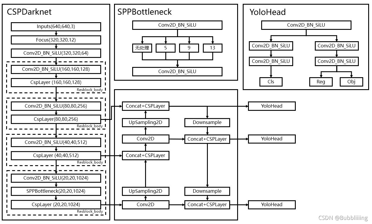
和之前版本的Yolo类似,整个YoloX可以依然可以分为三个部分,分别是CSPDarknet,FPN以及Yolo Head。
CSPDarknet可以被称作YoloX的主干特征提取网络,输入的图片首先会在CSPDarknet里面进行特征提取,提取到的特征可以被称作特征层,是输入图片的特征集合。在主干部分,我们获取了三个特征层进行下一步网络的构建,这三个特征层我称它为有效特征层。
FPN可以被称作YoloX的加强特征提取网络,在主干部分获得的三个有效特征层会在这一部分进行特征融合,特征融合的目的是结合不同尺度的特征信息。在FPN部分,已经获得的有效特征层被用于继续提取特征。在YoloX里面同样使用了YoloV4中用到的Panet的结构,我们不仅会对特征进行上采样实现特征融合,还会对特征再次进行下采样实现特征融合。
Yolo Head是YoloX的分类器与回归器,通过CSPDarknet和FPN,我们已经可以获得三个加强过的有效特征层。每一个特征层都有宽、高和通道数,此时我们可以将特征图看作一个又一个特征点的集合,每一个特征点都有通道数个特征。Yolo Head实际上所做的工作就是对特征点进行判断,判断特征点是否有物体与其对应。以前版本的Yolo所用的解耦头是一起的,也就是分类和回归在一个1X1卷积里实现,YoloX认为这给网络的识别带来了不利影响。在YoloX中,Yolo Head被分为了两部分,分别实现,最后预测的时候才整合在一起。
因此,整个YoloX网络所作的工作就是 特征提取-特征加强-预测特征点对应的物体情况。
二、网络结构解析
1、主干网络CSPDarknet介绍
YoloX所使用的主干特征提取网络为CSPDarknet,它具有五个重要特点:
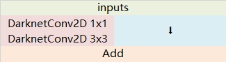
1、使用了残差网络Residual,CSPDarknet中的残差卷积可以分为两个部分,主干部分是一次1X1的卷积和一次3X3的卷积;残差边部分不做任何处理,直接将主干的输入与输出结合。整个YoloV3的主干部分都由残差卷积构成:
def Bottleneck(x, out_channels, shortcut=True, name = ""):
    y = compose(
            DarknetConv2D_BN_SiLU(out_channels, (1,1), name = name + '.conv1'),
            DarknetConv2D_BN_SiLU(out_channels, (3,3), name = name + '.conv2'))(x)
    if shortcut:
        y = Add()([x, y])
    return y
残差网络的特点是容易优化,并且能够通过增加相当的深度来提高准确率。其内部的残差块使用了跳跃连接,缓解了在深度神经网络中增加深度带来的梯度消失问题。
2、使用CSPnet网络结构,CSPnet结构并不算复杂,就是将原来的残差块的堆叠进行了一个拆分,拆成左右两部分:主干部分继续进行原来的残差块的堆叠;另一部分则像一个残差边一样,经过少量处理直接连接到最后。因此可以认为CSP中存在一个大的残差边。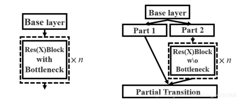
def CSPLayer(x, num_filters, num_blocks, shortcut=True, expansion=0.5, name=""):
    hidden_channels = int(num_filters * expansion)  # hidden channels
    #----------------------------------------------------------------#
    #   主干部分会对num_blocks进行循环,循环内部是残差结构。
    #----------------------------------------------------------------#
    x_1 = DarknetConv2D_BN_SiLU(hidden_channels, (1,1), name = name + '.conv1')(x)
    #--------------------------------------------------------------------#
    #   然后建立一个大的残差边shortconv、这个大残差边绕过了很多的残差结构
    #--------------------------------------------------------------------#
    x_2 = DarknetConv2D_BN_SiLU(hidden_channels, (1,1), name = name + '.conv2')(x)
    for i in range(num_blocks):
        x_1 = Bottleneck(x_1, hidden_channels, shortcut, name = name + '.m.' + str(i))
    #----------------------------------------------------------------#
    #   将大残差边再堆叠回来
    #----------------------------------------------------------------#
    route = Concatenate()([x_1, x_2])

    #----------------------------------------------------------------#
    #   最后对通道数进行整合
    #----------------------------------------------------------------#
    return DarknetConv2D_BN_SiLU(num_filters, (1,1), name = name + '.conv3')(route)
3、使用了Focus网络结构,这个网络结构是在YoloV5里面使用到比较有趣的网络结构,具体操作是在一张图片中每隔一个像素拿到一个值,这个时候获得了四个独立的特征层,然后将四个独立的特征层进行堆叠,此时宽高信息就集中到了通道信息,输入通道扩充了四倍。拼接起来的特征层相对于原先的三通道变成了十二个通道,下图很好的展示了Focus结构,一看就能明白。

class Focus(Layer):
    def __init__(self):
        super(Focus, self).__init__()

    def compute_output_shape(self, input_shape):
        return (input_shape[0], input_shape[1] // 2 if input_shape[1] != None else input_shape[1], input_shape[2] // 2 if input_shape[2] != None else input_shape[2], input_shape[3] * 4)

    def call(self, x):
        return tf.concat(
            [x[...,  ::2,  ::2, :],
             x[..., 1::2,  ::2, :],
             x[...,  ::2, 1::2, :],
             x[..., 1::2, 1::2, :]],
             axis=-1
        )
4、使用了SiLU激活函数,SiLU是Sigmoid和ReLU的改进版。SiLU具备无上界有下界、平滑、非单调的特性。SiLU在深层模型上的效果优于 ReLU。可以看做是平滑的ReLU激活函数。
f ( x ) = x ⋅ sigmoid ( x ) f(x) = x · \text{sigmoid}(x) f(x)=x⋅sigmoid(x)

class SiLU(Layer):
    def __init__(self, **kwargs):
        super(SiLU, self).__init__(**kwargs)
        self.supports_masking = True

    def call(self, inputs):
        return inputs * K.sigmoid(inputs)

    def get_config(self):
        config = super(SiLU, self).get_config()
        return config

    def compute_output_shape(self, input_shape):
        return input_shape
5、使用了SPP结构,通过不同池化核大小的最大池化进行特征提取,提高网络的感受野。在YoloV4中,SPP是用在FPN里面的,在YoloX中,SPP模块被用在了主干特征提取网络中。
def SPPBottleneck(x, out_channels, name = ""):
    #---------------------------------------------------#
    #   使用了SPP结构,即不同尺度的最大池化后堆叠。
    #---------------------------------------------------#
    x = DarknetConv2D_BN_SiLU(out_channels // 2, (1,1), name = name + '.conv1')(x)
    maxpool1 = MaxPooling2D(pool_size=(5,5), strides=(1,1), padding='same')(x)
    maxpool2 = MaxPooling2D(pool_size=(9,9), strides=(1,1), padding='same')(x)
    maxpool3 = MaxPooling2D(pool_size=(13,13), strides=(1,1), padding='same')(x)
    x = Concatenate()([x, maxpool1, maxpool2, maxpool3])
    x = DarknetConv2D_BN_SiLU(out_channels, (1,1), name = name + '.conv2')(x)
    return x
整个主干实现代码为:
from functools import wraps

import tensorflow as tf
from tensorflow.keras import backend as K
from tensorflow.keras.initializers import RandomNormal
from tensorflow.keras.layers import (Add, BatchNormalization, Concatenate,
                                     Conv2D, Layer, MaxPooling2D,
                                     ZeroPadding2D)
from tensorflow.keras.regularizers import l2
from utils.utils import compose


class SiLU(Layer):
    def __init__(self, **kwargs):
        super(SiLU, self).__init__(**kwargs)
        self.supports_masking = True

    def call(self, inputs):
        return inputs * K.sigmoid(inputs)

    def get_config(self):
        config = super(SiLU, self).get_config()
        return config

    def compute_output_shape(self, input_shape):
        return input_shape

class Focus(Layer):
    def __init__(self):
        super(Focus, self).__init__()

    def compute_output_shape(self, input_shape):
        return (input_shape[0], input_shape[1] // 2 if input_shape[1] != None else input_shape[1], input_shape[2] // 2 if input_shape[2] != None else input_shape[2], input_shape[3] * 4)

    def call(self, x):
        return tf.concat(
            [x[...,  ::2,  ::2, :],
             x[..., 1::2,  ::2, :],
             x[...,  ::2, 1::2, :],
             x[..., 1::2, 1::2, :]],
             axis=-1
        )
#------------------------------------------------------#
#   单次卷积DarknetConv2D
#   如果步长为2则自己设定padding方式。
#------------------------------------------------------#
@wraps(Conv2D)
def DarknetConv2D(*args, **kwargs):
    darknet_conv_kwargs = {

    'kernel_initializer' : random_normal(stddev=0.02)}
    darknet_conv_kwargs['padding'] = 'valid' if kwargs.get('strides')==(2,2) else 'same'
    darknet_conv_kwargs.update(kwargs)
    return Conv2D(*args, **darknet_conv_kwargs)

#---------------------------------------------------#
#   卷积块 -> 卷积 + 标准化 + 激活函数
#   DarknetConv2D + BatchNormalization + SiLU
#---------------------------------------------------#
def DarknetConv2D_BN_SiLU(*args, **kwargs):
    no_bias_kwargs = {

    'use_bias': False}
    no_bias_kwargs.update(kwargs)
    if "name" in kwargs.keys():
        no_bias_kwargs['name'] = kwargs['name'] + '.conv'
    return compose(
        DarknetConv2D(*args, **no_bias_kwargs),
        BatchNormalization(name = kwargs['name'] + '.bn'),
        SiLU())

def SPPBottleneck(x, out_channels, name = ""):
    #---------------------------------------------------#
    #   使用了SPP结构,即不同尺度的最大池化后堆叠。
    #---------------------------------------------------#
    x = DarknetConv2D_BN_SiLU(out_channels // 2, (1,1), name = name + '.conv1')(x)
    maxpool1 = MaxPooling2D(pool_size=(5,5), strides=(1,1), padding='same')(x)
    maxpool2 = MaxPooling2D(pool_size=(9,9), strides=(1,1), padding='same')(x)
    maxpool3 = MaxPooling2D(pool_size=(13,13), strides=(1,1), padding='same')(x)
    x = Concatenate()([x, maxpool1, maxpool2, maxpool3])
    x = DarknetConv2D_BN_SiLU(out_channels, (1,1), name = name + '.conv2')(x)
    return x

def Bottleneck(x, out_channels, shortcut=True, name = ""):
    y = compose(
            DarknetConv2D_BN_SiLU(out_channels, (1,1), name = name + '.conv1'),
            DarknetConv2D_BN_SiLU(out_channels, (3,3), name = name + '.conv2'))(x)
    if shortcut:
        y = Add()([x, y])
    return y

def CSPLayer(x, num_filters, num_blocks, shortcut=True, expansion=0.5, name=""):
    hidden_channels = int(num_filters * expansion)  # hidden channels
    #----------------------------------------------------------------#
    #   主干部分会对num_blocks进行循环,循环内部是残差结构。
    #----------------------------------------------------------------#
    x_1 = DarknetConv2D_BN_SiLU(hidden_channels, (1,1), name = name + '.conv1')(x)
    #--------------------------------------------------------------------#
    #   然后建立一个大的残差边shortconv、这个大残差边绕过了很多的残差结构
    #--------------------------------------------------------------------#
    x_2 = DarknetConv2D_BN_SiLU(hidden_channels, (1,1), name = name + '.conv2')(x)
    for i in range(num_blocks):
        x_1 = Bottleneck(x_1, hidden_channels, shortcut, name = name + '.m.' + str(i))
    #----------------------------------------------------------------#
    #   将大残差边再堆叠回来
    #----------------------------------------------------------------#
    route = Concatenate()([x_1, x_2])

    #----------------------------------------------------------------#
    #   最后对通道数进行整合
    #----------------------------------------------------------------#
    return DarknetConv2D_BN_SiLU(num_filters, (1,1), name = name + '.conv3')(route)

def resblock_body(x, num_filters, num_blocks, shortcut=True, expansion=0.5, last = False, name = ""):
    #----------------------------------------------------------------#
    #   利用ZeroPadding2D和一个步长为2x2的卷积块进行高和宽的压缩
    #----------------------------------------------------------------#
    x = ZeroPadding2D(((1,1),(1,1)))(x)
    #----------------------------------------------------------------#
    #   利用ZeroPadding2D和一个步长为2x2的卷积块进行高和宽的压缩
    #----------------------------------------------------------------#
    x = DarknetConv2D_BN_SiLU(num_filters, (3,3), strides=(2,2), name = name + '.0')(x)
    if last:
        x = SPPBottleneck(x, num_filters, name = name + '.1')
    return CSPLayer(x, num_filters, num_blocks, shortcut=shortcut, expansion=expansion, name = name + '.1' if not last else name + '.2')

#---------------------------------------------------#
#   CSPdarknet53 的主体部分
#   输入为一张416x416x3的图片
#   输出为三个有效特征层
#---------------------------------------------------#
def darknet_body(x, dep_mul, wid_mul):
    base_channels   = int(wid_mul * 64)  # 64
    base_depth      = max(round(dep_mul * 3), 1)  # 3

    x = Focus()(x)
    x = DarknetConv2D_BN_SiLU(base_channels, (3,3), name = 'backbone.backbone.stem.conv')(x)

    x = resblock_body(x, base_channels * 2, base_depth, name = 'backbone.backbone.dark2')
    x = resblock_body(x, base_channels * 4, base_depth * 3, name = 'backbone.backbone.dark3')
    feat1 = x
    x = resblock_body(x, base_channels * 8, base_depth * 3, name = 'backbone.backbone.dark4')
    feat2 = x
    x = resblock_body(x, base_channels * 16, base_depth, last = True, name = 'backbone.backbone.dark5')
    feat3 = x
    return feat1,feat2,feat3
2、构建FPN特征金字塔进行加强特征提取

在特征利用部分,YoloX提取多特征层进行目标检测,一共提取三个特征层。
三个特征层位于主干部分CSPdarknet的不同位置,分别位于中间层,中下层,底层,当输入为(640,640,3)的时候,三个特征层的shape分别为feat1=(80,80,256)、feat2=(40,40,512)、feat3=(20,20,1024)。
在获得三个有效特征层后,我们利用这三个有效特征层进行FPN层的构建,构建方式为:
- feat3=(20,20,1024)的特征层进行1次1X1卷积调整通道后获得P5,P5进行上采样UmSampling2d后与feat2=(40,40,512)特征层进行结合,然后使用CSPLayer进行特征提取获得P5_upsample,此时获得的特征层为(40,40,512)。
- P5_upsample=(40,40,512)的特征层进行1次1X1卷积调整通道后获得P4,P4进行上采样UmSampling2d后与feat1=(80,80,256)特征层进行结合,然后使用CSPLayer进行特征提取P3_out,此时获得的特征层为(80,80,256)。
- P3_out=(80,80,256)的特征层进行一次3x3卷积进行下采样,下采样后与P4堆叠,然后使用CSPLayer进行特征提取P4_out,此时获得的特征层为(40,40,512)。
- P4_out=(40,40,512)的特征层进行一次3x3卷积进行下采样,下采样后与P5堆叠,然后使用CSPLayer进行特征提取P5_out,此时获得的特征层为(20,20,1024)。
特征金字塔可以将不同shape的特征层进行特征融合,有利于提取出更好的特征。
from tensorflow.keras.layers import (Concatenate, Input, Lambda, UpSampling2D,
                          ZeroPadding2D)
from tensorflow.keras.models import Model

from nets.CSPdarknet import (CSPLayer, DarknetConv2D, DarknetConv2D_BN_SiLU,
                               darknet_body)
from nets.yolo_training import get_yolo_loss

#---------------------------------------------------#
#   Panet网络的构建,并且获得预测结果
#---------------------------------------------------#
def yolo_body(input_shape, num_classes, phi):
    depth_dict      = {

    's' : 0.33, 'm' : 0.67, 'l' : 1.00, 'x' : 1.33,}
    width_dict      = {

    's' : 0.50, 'm' : 0.75, 'l' : 1.00, 'x' : 1.25,}
    depth, width    = depth_dict[phi], width_dict[phi]
    in_channels     = [256, 512, 1024]

    inputs      = Input(input_shape)
    feat1, feat2, feat3 = darknet_body(inputs, depth, width)

    P5          = DarknetConv2D_BN_SiLU(int(in_channels[1] * width), (1, 1), name = 'backbone.lateral_conv0')(feat3)
    P5_upsample = UpSampling2D()(P5)  # 512/16
    P5_upsample = Concatenate(axis = -1)([P5_upsample, feat2])  # 512->1024/16
    P5_upsample = CSPLayer(P5_upsample, int(in_channels[1] * width), round(3 * depth), shortcut = False, name = 'backbone.C3_p4')  # 1024->512/16

    P4          = DarknetConv2D_BN_SiLU(int(in_channels[0] * width), (1, 1), name = 'backbone.reduce_conv1')(P5_upsample)  # 512->256/16
    P4_upsample = UpSampling2D()(P4)  # 256/8
    P4_upsample = Concatenate(axis = -1)([P4_upsample, feat1])  # 256->512/8
    P3_out      = CSPLayer(P4_upsample, int(in_channels[0] * width), round(3 * depth), shortcut = False, name = 'backbone.C3_p3')  # 1024->512/16

    P3_downsample   = ZeroPadding2D(((1,1),(1,1)))(P3_out)
    P3_downsample   = DarknetConv2D_BN_SiLU(int(in_channels[0] * width), (3, 3), strides = (2, 2), name = 'backbone.bu_conv2')(P3_downsample)  # 256->256/16
    P3_downsample   = Concatenate(axis = -1)([P3_downsample, P4])  # 256->512/16
    P4_out          = CSPLayer(P3_downsample, int(in_channels[1] * width), round(3 * depth), shortcut = False, name = 'backbone.C3_n3')  # 1024->512/16

    P4_downsample   = ZeroPadding2D(((1,1),(1,1)))(P4_out)
    P4_downsample   = DarknetConv2D_BN_SiLU(int(in_channels[1] * width), (3, 3), strides = (2, 2), name = 'backbone.bu_conv1')(P4_downsample)  # 256->256/16
    P4_downsample   = Concatenate(axis = -1)([P4_downsample, P5])  # 512->1024/32
    P5_out          = CSPLayer(P4_downsample, int(in_channels[2] * width), round(3 * depth), shortcut = False, name = 'backbone.C3_n4')  # 1024->512/16
3、利用Yolo Head获得预测结果
利用FPN特征金字塔,我们可以获得三个加强特征,这三个加强特征的shape分别为(20,20,1024)、(40,40,512)、(80,80,256),然后我们利用这三个shape的特征层传入Yolo Head获得预测结果。
YoloX中的YoloHead与之前版本的YoloHead不同。以前版本的Yolo所用的解耦头是一起的,也就是分类和回归在一个1X1卷积里实现,YoloX认为这给网络的识别带来了不利影响。在YoloX中,Yolo Head被分为了两部分,分别实现,最后预测的时候才整合在一起。
 对于每一个特征层,我们可以获得三个预测结果,分别是:
1、Reg(h,w,4)用于判断每一个特征点的回归参数,回归参数调整后可以获得预测框。
2、Obj(h,w,1)用于判断每一个特征点是否包含物体。
3、Cls(h,w,num_classes)用于判断每一个特征点所包含的物体种类。
将三个预测结果进行堆叠,每个特征层获得的结果为:
Out(h,w,4+1+num_classses)前四个参数用于判断每一个特征点的回归参数,回归参数调整后可以获得预测框;第五个参数用于判断每一个特征点是否包含物体;最后num_classes个参数用于判断每一个特征点所包含的物体种类。
实现代码如下:
fpn_outs    = [P3_out, P4_out, P5_out]
yolo_outs   = []
for i, out in enumerate(fpn_outs):
    stem    = DarknetConv2D_BN_SiLU(int(256 * width), (1, 1), strides = (1, 1), name = 'head.stems.' + str(i))(out)

    cls_conv = DarknetConv2D_BN_SiLU(int(256 * width), (3, 3), strides = (1, 1), name = 'head.cls_convs.' + str(i) + '.0')(stem)
    cls_conv = DarknetConv2D_BN_SiLU(int(256 * width), (3, 3), strides = (1, 1), name = 'head.cls_convs.' + str(i) + '.1')(cls_conv)
    cls_pred = DarknetConv2D(num_classes, (1, 1), strides = (1, 1), name = 'head.cls_preds.' + str(i))(cls_conv)

    reg_conv = DarknetConv2D_BN_SiLU(int(256 * width), (3, 3), strides = (1, 1), name = 'head.reg_convs.' + str(i) + '.0')(stem)
    reg_conv = DarknetConv2D_BN_SiLU(int(256 * width), (3, 3), strides = (1, 1), name = 'head.reg_convs.' + str(i) + '.1')(reg_conv)
    reg_pred = DarknetConv2D(4, (1, 1), strides = (1, 1), name = 'head.reg_preds.' + str(i))(reg_conv)
    obj_pred = DarknetConv2D(1, (1, 1), strides = (1, 1), name = 'head.obj_preds.' + str(i))(reg_conv)
    output   = Concatenate(axis = -1)([reg_pred, obj_pred, cls_pred])
    yolo_outs.append(output)
return Model(inputs, yolo_outs)
三、预测结果的解码
1、获得预测框与得分
在对预测结果进行解码之前,我们再来看看预测结果代表了什么,预测结果可以分为3个部分:
通过上一步,我们获得了每个特征层的三个预测结果。
本文以(20,20,1024)对应的三个预测结果为例:
1、Reg预测结果,此时卷积的通道数为4,最终结果为(20,20,4)。其中的4可以分为两个2,第一个2是预测框的中心点相较于该特征点的偏移情况,第二个2是预测框的宽高相较于对数指数的参数
2、Obj预测结果,此时卷积的通道数为1,最终结果为(20,20,1),代表每一个特征点预测框内部包含物体的概率。
3、Cls预测结果,此时卷积的通道数为num_classes,最终结果为(20,20,num_classes),代表每一个特征点对应某类物体的概率,最后一维度num_classes中的预测值代表属于每一个类的概率;
该特征层相当于将图像划分成20x20个特征点,如果某个特征点落在物体的对应框内,就用于预测该物体。
如图所示,蓝色的点为20x20的特征点,此时我们对左图红色的三个点进行解码操作演示:
1、进行中心预测点的计算,利用Regression预测结果前两个序号的内容对特征点坐标进行偏移,左图红色的三个特征点偏移后是右图绿色的三个点;
2、进行预测框宽高的计算,利用Regression预测结果后两个序号的内容求指数后获得预测框的宽高;
3、此时获得的预测框就可以绘制在图片上了。

除去这样的解码操作,还有非极大抑制的操作需要进行,防止同一种类的框的堆积。
#---------------------------------------------------#
#   图片预测
#---------------------------------------------------#
def DecodeBox(outputs,
            num_classes,
            image_shape,
            input_shape,
            max_boxes       = 100,
            confidence      = 0.5,
            nms_iou         = 0.3,
            letterbox_image = True):

    bs      = K.shape(outputs[0])[0]

    grids   = []
    strides = []
    hw      = [K.shape(x)[1:3] for x in outputs]
    outputs = tf.concat([tf.reshape(x, [bs, -1, 5 + num_classes]) for x in outputs], axis = 1)
    for i in range(len(hw)):
        #---------------------------#
        #   根据特征层生成网格点
        #---------------------------#
        grid_x, grid_y  = tf.meshgrid(K.arange(hw[i][1]), K.arange(hw[i][0]))
        grid            = tf.reshape(tf.stack((grid_x, grid_y), 2), (1, -1, 2))
        shape           = tf.shape(grid)[:2]

        grids.append(tf.cast(grid, K.dtype(outputs)))
        strides.append(tf.ones((shape[0], shape[1], 1)) * input_shape[0] / tf.cast(hw[i][0], K.dtype(outputs)))
    #---------------------------#
    #   将网格点堆叠到一起
    #---------------------------#
    grids               = tf.concat(grids, axis=1)
    strides             = tf.concat(strides, axis=1)
    #------------------------#
    #   根据网格点进行解码
    #------------------------#
    box_xy = (outputs[..., :2] + grids) * strides / K.cast(input_shape[::-1], K.dtype(outputs))
    box_wh = tf.exp(outputs[..., 2:4]) * strides / K.cast(input_shape[::-1], K.dtype(outputs))

    box_confidence  = K.sigmoid(outputs[..., 4:5])
    box_class_probs = K.sigmoid(outputs[..., 5: ])
    #------------------------------------------------------------------------------------------------------------#
    #   在图像传入网络预测前会进行letterbox_image给图像周围添加灰条,因此生成的box_xy, box_wh是相对于有灰条的图像的
    #   我们需要对其进行修改,去除灰条的部分。 将box_xy、和box_wh调节成y_min,y_max,xmin,xmax
    #   如果没有使用letterbox_image也需要将归一化后的box_xy, box_wh调整成相对于原图大小的
    #------------------------------------------------------------------------------------------------------------#
    boxes       = yolo_correct_boxes(box_xy, box_wh, input_shape, image_shape, letterbox_image)
2、得分筛选与非极大抑制
得到最终的预测结果后还要进行得分排序与非极大抑制筛选。
得分筛选就是筛选出得分满足confidence置信度的预测框。
非极大抑制就是筛选出一定区域内属于同一种类得分最大的框。
得分筛选与非极大抑制的过程可以概括如下:
1、找出该图片中得分大于门限函数的框。在进行重合框筛选前就进行得分的筛选可以大幅度减少框的数量。
2、对种类进行循环,非极大抑制的作用是筛选出一定区域内属于同一种类得分最大的框,对种类进行循环可以帮助我们对每一个类分别进行非极大抑制。
3、根据得分对该种类进行从大到小排序。
4、每次取出得分最大的框,计算其与其它所有预测框的重合程度,重合程度过大的则剔除。
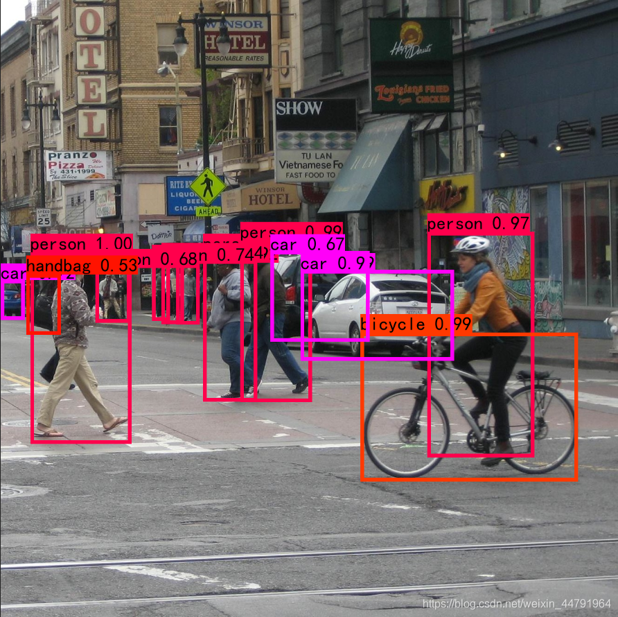
得分筛选与非极大抑制后的结果就可以用于绘制预测框了。
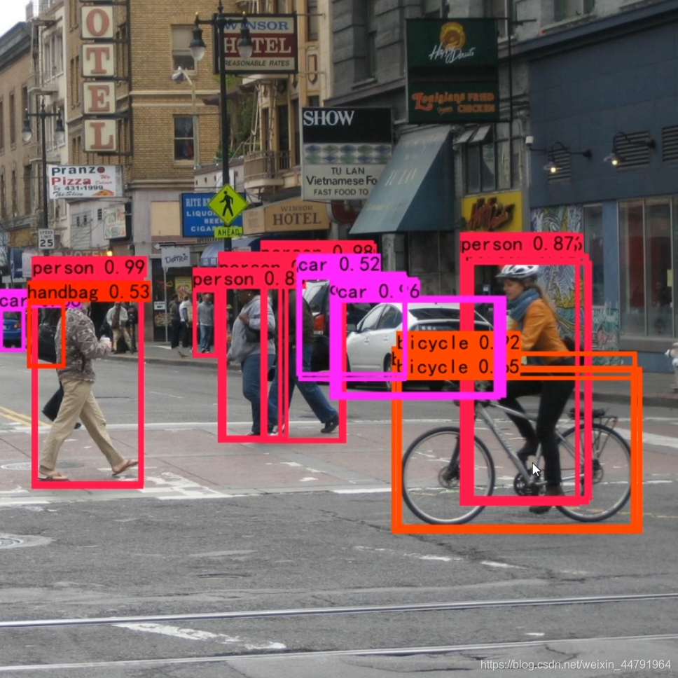
下图是经过非极大抑制的。
下图是未经过非极大抑制的。
实现代码为:
box_scores  = box_confidence * box_class_probs

#-----------------------------------------------------------#
#   判断得分是否大于score_threshold
#-----------------------------------------------------------#
mask             = box_scores >= confidence
max_boxes_tensor = K.constant(max_boxes, dtype='int32')
boxes_out   = []
scores_out  = []
classes_out = []
for c in range(num_classes):
    #-----------------------------------------------------------#
    #   取出所有box_scores >= score_threshold的框,和成绩
    #-----------------------------------------------------------#
    class_boxes      = tf.boolean_mask(boxes, mask[:, c])
    class_box_scores = tf.boolean_mask(box_scores[:, c], mask[:, c])

    #-----------------------------------------------------------#
    #   非极大抑制
    #   保留一定区域内得分最大的框
    #-----------------------------------------------------------#
    nms_index = tf.image.non_max_suppression(class_boxes, class_box_scores, max_boxes_tensor, iou_threshold=nms_iou)

    #-----------------------------------------------------------#
    #   获取非极大抑制后的结果
    #   下列三个分别是:框的位置,得分与种类
    #-----------------------------------------------------------#
    class_boxes         = K.gather(class_boxes, nms_index)
    class_box_scores    = K.gather(class_box_scores, nms_index)
    classes             = K.ones_like(class_box_scores, 'int32') * c

    boxes_out.append(class_boxes)
    scores_out.append(class_box_scores)
    classes_out.append(classes)
boxes_out      = K.concatenate(boxes_out, axis=0)
scores_out     = K.concatenate(scores_out, axis=0)
classes_out    = K.concatenate(classes_out, axis=0)
四、训练部分
1、计算loss所需内容
计算loss实际上是网络的预测结果和网络的真实结果的对比。
和网络的预测结果一样,网络的损失也由三个部分组成,分别是Reg部分、Obj部分、Cls部分。Reg部分是特征点的回归参数判断、Obj部分是特征点是否包含物体判断、Cls部分是特征点包含的物体的种类。
2、正样本特征点的必要条件
在YoloX中,物体的真实框落在哪些特征点内就由该特征点来预测。
对于每一个真实框,我们会求取所有特征点与它的空间位置情况。作为正样本的特征点需要满足以下几个特点:
1、特征点落在物体的真实框内。
2、特征点距离物体中心尽量要在一定半径内。
特点1、2保证了属于正样本的特征点会落在物体真实框内部,特征点中心与物体真实框中心要相近。
上面两个条件仅用作正样本的而初步筛选,在YoloX中,我们使用了SimOTA方法进行动态的正样本数量分配。
def get_in_boxes_info(gt_bboxes_per_image, x_shifts, y_shifts, expanded_strides, num_gt, total_num_anchors, center_radius = 2.5):
    #-------------------------------------------------------#
    #   expanded_strides_per_image  [n_anchors_all]
    #   x_centers_per_image         [num_gt, n_anchors_all]
    #   x_centers_per_image         [num_gt, n_anchors_all]
    #-------------------------------------------------------#
    expanded_strides_per_image  = expanded_strides[0]
    x_centers_per_image         = tf.tile(tf.expand_dims(((x_shifts[0] + 0.5) * expanded_strides_per_image), 0), [num_gt, 1])
    y_centers_per_image         = tf.tile(tf.expand_dims(((y_shifts[0] + 0.5) * expanded_strides_per_image), 0), [num_gt, 1])

    #-------------------------------------------------------#
    #   gt_bboxes_per_image_x       [num_gt, n_anchors_all]
    #-------------------------------------------------------#
    gt_bboxes_per_image_l = tf.tile(tf.expand_dims((gt_bboxes_per_image[:, 0] - 0.5 * gt_bboxes_per_image[:, 2]), 1), [1, total_num_anchors])
    gt_bboxes_per_image_r = tf.tile(tf.expand_dims((gt_bboxes_per_image[:, 0] + 0.5 * gt_bboxes_per_image[:, 2]), 1), [1, total_num_anchors])
    gt_bboxes_per_image_t = tf.tile(tf.expand_dims((gt_bboxes_per_image[:, 1] - 0.5 * gt_bboxes_per_image[:, 3]), 1), [1, total_num_anchors])
    gt_bboxes_per_image_b = tf.tile(tf.expand_dims((gt_bboxes_per_image[:, 1] + 0.5 * gt_bboxes_per_image[:, 3]), 1), [1, total_num_anchors])

    #-------------------------------------------------------#
    #   bbox_deltas     [num_gt, n_anchors_all, 4]
    #-------------------------------------------------------#
    b_l = x_centers_per_image - gt_bboxes_per_image_l
    b_r = gt_bboxes_per_image_r - x_centers_per_image
    b_t = y_centers_per_image - gt_bboxes_per_image_t
    b_b = gt_bboxes_per_image_b - y_centers_per_image
    bbox_deltas = tf.stack([b_l, b_t, b_r, b_b], 2)

    #-------------------------------------------------------#
    #   is_in_boxes     [num_gt, n_anchors_all]
    #   is_in_boxes_all [n_anchors_all]
    #-------------------------------------------------------#
    is_in_boxes     = tf.reduce_min(bbox_deltas, axis = -1) > 0.0
    is_in_boxes_all = tf.reduce_sum(tf.cast(is_in_boxes, K.dtype(gt_bboxes_per_image)), axis = 0) > 0.0

    gt_bboxes_per_image_l = tf.tile(tf.expand_dims(gt_bboxes_per_image[:, 0], 1), [1, total_num_anchors]) - center_radius * tf.expand_dims(expanded_strides_per_image, 0)
    gt_bboxes_per_image_r = tf.tile(tf.expand_dims(gt_bboxes_per_image[:, 0], 1), [1, total_num_anchors]) + center_radius * tf.expand_dims(expanded_strides_per_image, 0)
    gt_bboxes_per_image_t = tf.tile(tf.expand_dims(gt_bboxes_per_image[:, 1], 1), [1, total_num_anchors]) - center_radius * tf.expand_dims(expanded_strides_per_image, 0)
    gt_bboxes_per_image_b = tf.tile(tf.expand_dims(gt_bboxes_per_image[:, 1], 1), [1, total_num_anchors]) + center_radius * tf.expand_dims(expanded_strides_per_image, 0)

    #-------------------------------------------------------#
    #   center_deltas   [num_gt, n_anchors_all, 4]
    #-------------------------------------------------------#
    c_l = x_centers_per_image - gt_bboxes_per_image_l
    c_r = gt_bboxes_per_image_r - x_centers_per_image
    c_t = y_centers_per_image - gt_bboxes_per_image_t
    c_b = gt_bboxes_per_image_b - y_centers_per_image
    center_deltas       = tf.stack([c_l, c_t, c_r, c_b], 2)

    #-------------------------------------------------------#
    #   is_in_centers       [num_gt, n_anchors_all]
    #   is_in_centers_all   [n_anchors_all]
    #-------------------------------------------------------#
    is_in_centers       = tf.reduce_min(center_deltas, axis = -1) > 0.0
    is_in_centers_all   = tf.reduce_sum(tf.cast(is_in_centers, K.dtype(gt_bboxes_per_image)), axis = 0) > 0.0

    #-------------------------------------------------------#
    #   fg_mask                 [n_anchors_all]
    #   is_in_boxes_and_center  [num_gt, fg_mask]
    #-------------------------------------------------------#
    fg_mask = tf.cast(is_in_boxes_all | is_in_centers_all, tf.bool)

    is_in_boxes_and_center  = tf.boolean_mask(is_in_boxes, fg_mask, axis = 1) & tf.boolean_mask(is_in_centers, fg_mask, axis = 1)
    return fg_mask, is_in_boxes_and_center
3、SimOTA动态匹配正样本
在YoloX中,我们会计算一个Cost代价矩阵,代表每个真实框和每个特征点之间的代价关系,Cost代价矩阵由三个部分组成:
1、每个真实框和当前特征点预测框的重合程度;
2、每个真实框和当前特征点预测框的种类预测准确度;
3、每个真实框的中心是否落在了特征点的一定半径内。
每个真实框和当前特征点预测框的重合程度越高,代表这个特征点已经尝试去拟合该真实框了,因此它的Cost代价就会越小。
每个真实框和当前特征点预测框的种类预测准确度越高,也代表这个特征点已经尝试去拟合该真实框了,因此它的Cost代价就会越小。
每个真实框的中心如果落在了特征点的一定半径内,代表这个特征点应该去拟合该真实框,因此它的Cost代价就会越小。
Cost代价矩阵的目的是自适应的找到当前特征点应该去拟合的真实框,重合度越高越需要拟合,分类越准越需要拟合,在一定半径内越需要拟合。
在SimOTA中,不同目标设定不同的正样本数量(dynamick),以旷视科技官方回答中的蚂蚁和西瓜为例子,传统的正样本分配方案常常为同一场景下的西瓜和蚂蚁分配同样的正样本数,那要么蚂蚁有很多低质量的正样本,要么西瓜仅仅只有一两个正样本。对于哪个分配方式都是不合适的。
动态的正样本设置的关键在于如何确定k,SimOTA具体的做法是首先计算每个目标Cost最低的10特征点,然后把这十个特征点对应的预测框与真实框的IOU加起来求得最终的k。
因此,SimOTA的过程总结如下:
1、计算每个真实框和当前特征点预测框的重合程度。
2、计算将重合度最高的十个预测框与真实框的IOU加起来求得每个真实框的k,也就代表每个真实框有k个特征点与之对应。
3、计算每个真实框和当前特征点预测框的种类预测准确度。
4、判断真实框的中心是否落在了特征点的一定半径内。
5、计算Cost代价矩阵。
6、将Cost最低的k个点作为该真实框的正样本。
def get_assignments(gt_bboxes_per_image, gt_classes, bboxes_preds_per_image, obj_preds_per_image, cls_preds_per_image, x_shifts, y_shifts, expanded_strides, num_classes, num_gt, total_num_anchors):
    #-------------------------------------------------------#
    #   fg_mask                 [n_anchors_all]
    #   is_in_boxes_and_center  [num_gt, len(fg_mask)]
    #-------------------------------------------------------#
    fg_mask, is_in_boxes_and_center = get_in_boxes_info(gt_bboxes_per_image, x_shifts, y_shifts, expanded_strides, num_gt, total_num_anchors)

    #-------------------------------------------------------#
    #   fg_mask                 [n_anchors_all]
    #   bboxes_preds_per_image  [fg_mask, 4]
    #   cls_preds_              [fg_mask, num_classes]
    #   obj_preds_              [fg_mask, 1]
    #-------------------------------------------------------#
    bboxes_preds_per_image  = tf.boolean_mask(bboxes_preds_per_image, fg_mask, axis = 0)
    obj_preds_              = tf.boolean_mask(obj_preds_per_image, fg_mask, axis = 0)
    cls_preds_              = tf.boolean_mask(cls_preds_per_image, fg_mask, axis = 0)
    num_in_boxes_anchor     = tf.shape(bboxes_preds_per_image)[0]

    #-------------------------------------------------------#
    #   pair_wise_ious      [num_gt, fg_mask]
    #-------------------------------------------------------#
    pair_wise_ious      = bboxes_iou(gt_bboxes_per_image, bboxes_preds_per_image)
    pair_wise_ious_loss = -tf.log(pair_wise_ious + 1e-8)
    #-------------------------------------------------------#
    #   cls_preds_          [num_gt, fg_mask, num_classes]
    #   gt_cls_per_image    [num_gt, fg_mask, num_classes]
    #-------------------------------------------------------#
    gt_cls_per_image    = tf.tile(tf.expand_dims(tf.one_hot(tf.cast(gt_classes, tf.int32), num_classes), 1), (1, num_in_boxes_anchor, 1))
    cls_preds_          = K.sigmoid(tf.tile(tf.expand_dims(cls_preds_, 0), (num_gt, 1, 1))) *\
                          K.sigmoid(tf.tile(tf.expand_dims(obj_preds_, 0), (num_gt, 1, 1)))

    pair_wise_cls_loss  = tf.reduce_sum(K.binary_crossentropy(gt_cls_per_image, tf.sqrt(cls_preds_)), -1)

    cost = pair_wise_cls_loss + 3.0 * pair_wise_ious_loss + 100000.0 * tf.cast((~is_in_boxes_and_center), K.dtype(bboxes_preds_per_image))

    gt_matched_classes, fg_mask, pred_ious_this_matching, matched_gt_inds, num_fg = dynamic_k_matching(cost, pair_wise_ious, fg_mask, gt_classes, num_gt)
    return gt_matched_classes, fg_mask, pred_ious_this_matching, matched_gt_inds, num_fg

def bboxes_iou(b1, b2):
    #---------------------------------------------------#
    #   num_anchor,1,4
    #   计算左上角的坐标和右下角的坐标
    #---------------------------------------------------#
    b1              = K.expand_dims(b1, -2)
    b1_xy           = b1[..., :2]
    b1_wh           = b1[..., 2:4]
    b1_wh_half      = b1_wh/2.
    b1_mins         = b1_xy - b1_wh_half
    b1_maxes        = b1_xy + b1_wh_half

    #---------------------------------------------------#
    #   1,n,4
    #   计算左上角和右下角的坐标
    #---------------------------------------------------#
    b2              = K.expand_dims(b2, 0)
    b2_xy           = b2[..., :2]
    b2_wh           = b2[..., 2:4]
    b2_wh_half      = b2_wh/2.
    b2_mins         = b2_xy - b2_wh_half
    b2_maxes        = b2_xy + b2_wh_half

    #---------------------------------------------------#
    #   计算重合面积
    #---------------------------------------------------#
    intersect_mins  = K.maximum(b1_mins, b2_mins)
    intersect_maxes = K.minimum(b1_maxes, b2_maxes)
    intersect_wh    = K.maximum(intersect_maxes - intersect_mins, 0.)
    intersect_area  = intersect_wh[..., 0] * intersect_wh[..., 1]
    b1_area         = b1_wh[..., 0] * b1_wh[..., 1]
    b2_area         = b2_wh[..., 0] * b2_wh[..., 1]
    iou             = intersect_area / (b1_area + b2_area - intersect_area)
    return iou

def dynamic_k_matching(cost, pair_wise_ious, fg_mask, gt_classes, num_gt):
    #-------------------------------------------------------#
    #   cost                [num_gt, fg_mask]
    #   pair_wise_ious      [num_gt, fg_mask]
    #   gt_classes          [num_gt]
    #   fg_mask             [n_anchors_all]
    #   matching_matrix     [num_gt, fg_mask]
    #-------------------------------------------------------#
    matching_matrix         = tf.zeros_like(cost)

    #------------------------------------------------------------#
    #   选取iou最大的n_candidate_k个点
    #   然后求和,判断应该有多少点用于该框预测
    #   topk_ious           [num_gt, n_candidate_k]
    #   dynamic_ks          [num_gt]
    #   matching_matrix     [num_gt, fg_mask]
    #------------------------------------------------------------#
    n_candidate_k           = tf.minimum(10, tf.shape(pair_wise_ious)[1])
    topk_ious, _            = tf.nn.top_k(pair_wise_ious, n_candidate_k)
    dynamic_ks              = tf.maximum(tf.reduce_sum(topk_ious, 1), 1)
    # dynamic_ks              = tf.Print(dynamic_ks, [topk_ious, dynamic_ks], summarize = 100)

    def loop_body_1(b, matching_matrix):
        #------------------------------------------------------------#
        #   给每个真实框选取最小的动态k个点
        #------------------------------------------------------------#
        _, pos_idx = tf.nn.top_k(-cost[b], k=tf.cast(dynamic_ks[b], tf.int32))
        matching_matrix = tf.concat(
            [matching_matrix[:b], tf.expand_dims(tf.reduce_max(tf.one_hot(pos_idx, tf.shape(cost)[1]), 0), 0), matching_matrix[b+1:]], axis = 0
        )
        # matching_matrix = matching_matrix.write(b, K.cast(tf.reduce_max(tf.one_hot(pos_idx, tf.shape(cost)[1]), 0), K.dtype(cost)))
        return b + 1, matching_matrix
    #-----------------------------------------------------------#
    #   在这个地方进行一个循环、循环是对每一张图片进行的
    #-----------------------------------------------------------#
    _, matching_matrix = K.control_flow_ops.while_loop(lambda b,*args: b < tf.cast(num_gt, tf.int32), loop_body_1, [0, matching_matrix])

    #------------------------------------------------------------#
    #   anchor_matching_gt  [fg_mask]
    #------------------------------------------------------------#
    anchor_matching_gt = tf.reduce_sum(matching_matrix, 0)
    #------------------------------------------------------------#
    #   当某一个特征点指向多个真实框的时候
    #   选取cost最小的真实框。
    #------------------------------------------------------------#
    biger_one_indice = tf.reshape(tf.where(anchor_matching_gt > 1), [-1])
    def loop_body_2(b, matching_matrix):
        indice_anchor   = tf.cast(biger_one_indice[b], tf.int32)
        indice_gt       = tf.math.argmin(cost[:, indice_anchor])
        matching_matrix = tf.concat(
            [
                matching_matrix[:, :indice_anchor],
                tf.expand_dims(tf.one_hot(indice_gt, tf.cast(num_gt, tf.int32)), 1),
                matching_matrix[:, indice_anchor+1:]
            ], axis = -1
        )
        return b + 1, matching_matrix
    #-----------------------------------------------------------#
    #   在这个地方进行一个循环、循环是对每一张图片进行的
    #-----------------------------------------------------------#
    _, matching_matrix = K.control_flow_ops.while_loop(lambda b,*args: b < tf.cast(tf.shape(biger_one_indice)[0], tf.int32), loop_body_2, [0, matching_matrix])

    #------------------------------------------------------------#
    #   fg_mask_inboxes  [fg_mask]
    #   num_fg为正样本的特征点个数
    #------------------------------------------------------------#
    fg_mask_inboxes = tf.reduce_sum(matching_matrix, 0) > 0.0
    num_fg          = tf.reduce_sum(tf.cast(fg_mask_inboxes, K.dtype(cost)))

    fg_mask_indices         = tf.reshape(tf.where(fg_mask), [-1])
    fg_mask_inboxes_indices = tf.reshape(tf.where(fg_mask_inboxes), [-1, 1])
    fg_mask_select_indices  = tf.gather_nd(fg_mask_indices, fg_mask_inboxes_indices)
    fg_mask                 = tf.cast(tf.reduce_max(tf.one_hot(fg_mask_select_indices, tf.shape(fg_mask)[0]), 0), K.dtype(fg_mask))

    #------------------------------------------------------------#
    #   获得特征点对应的物品种类
    #------------------------------------------------------------#
    matched_gt_inds     = tf.math.argmax(tf.boolean_mask(matching_matrix, fg_mask_inboxes, axis = 1), 0)
    gt_matched_classes  = tf.gather_nd(gt_classes, tf.reshape(matched_gt_inds, [-1, 1]))

    pred_ious_this_matching = tf.boolean_mask(tf.reduce_sum(matching_matrix * pair_wise_ious, 0), fg_mask_inboxes)
    return gt_matched_classes, fg_mask, pred_ious_this_matching, matched_gt_inds, num_fg
4、计算Loss
由第一部分可知,YoloX的损失由三个部分组成:
1、Reg部分,由第三部分可知道每个真实框对应的特征点,获取到每个框对应的特征点后,取出该特征点的预测框,利用真实框和预测框计算IOU损失,作为Reg部分的Loss组成。
2、Obj部分,由第三部分可知道每个真实框对应的特征点,所有真实框对应的特征点都是正样本,剩余的特征点均为负样本,根据正负样本和特征点的是否包含物体的预测结果计算交叉熵损失,作为Obj部分的Loss组成。
3、Cls部分,由第三部分可知道每个真实框对应的特征点,获取到每个框对应的特征点后,取出该特征点的种类预测结果,根据真实框的种类和特征点的种类预测结果计算交叉熵损失,作为Cls部分的Loss组成。
def get_yolo_loss(input_shape, num_layers, num_classes):
    def yolo_loss(args):
        labels, y_pred = args[-1], args[:-1]
        x_shifts            = []
        y_shifts            = []
        expanded_strides    = []
        outputs             = []
        #-----------------------------------------------#
        # inputs    [[batch_size, 20, 20, num_classes + 5]
        #            [batch_size, 40, 40, num_classes + 5]
        #            [batch_size, 80, 80, num_classes + 5]]
        # outputs   [[batch_size, 400, num_classes + 5]
        #            [batch_size, 1600, num_classes + 5]
        #            [batch_size, 6400, num_classes + 5]]
        #-----------------------------------------------#
        for i in range(num_layers):
            output          = y_pred[i]
            grid_shape      = tf.shape(output)[1:3]
            stride          = input_shape[0] / tf.cast(grid_shape[0], K.dtype(output))

            grid_x, grid_y  = tf.meshgrid(K.arange(grid_shape[1]), K.arange(grid_shape[0]))
            grid            = tf.cast(tf.reshape(tf.stack((grid_x, grid_y), 2), (1, -1, 2)), K.dtype(output))

            output          = tf.reshape(output, [tf.shape(y_pred[i])[0], grid_shape[0] * grid_shape[1], -1])
            output_xy       = (output[..., :2] + grid) * stride
            output_wh       = tf.exp(output[..., 2:4]) * stride
            output          = tf.concat([output_xy, output_wh, output[..., 4:]], -1)

            x_shifts.append(grid[..., 0])
            y_shifts.append(grid[..., 1])
            expanded_strides.append(tf.ones_like(grid[..., 0]) * stride)
            outputs.append(output)
        #-----------------------------------------------#
        #   x_shifts            [1, n_anchors_all]
        #   y_shifts            [1, n_anchors_all]
        #   expanded_strides    [1, n_anchors_all]
        #-----------------------------------------------#
        x_shifts            = tf.concat(x_shifts, 1)
        y_shifts            = tf.concat(y_shifts, 1)
        expanded_strides    = tf.concat(expanded_strides, 1)
        outputs             = tf.concat(outputs, 1)
        return get_losses(x_shifts, y_shifts, expanded_strides, outputs, labels, num_classes)
    return yolo_loss

def get_losses(x_shifts, y_shifts, expanded_strides, outputs, labels, num_classes):
    #-----------------------------------------------#
    #   [batch, n_anchors_all, 4]
    #   [batch, n_anchors_all, 1]
    #   [batch, n_anchors_all, n_cls]
    #-----------------------------------------------#
    bbox_preds  = outputs[:, :, :4]
    obj_preds   = outputs[:, :, 4:5]
    cls_preds   = outputs[:, :, 5:]

    #------------------------------------------------------------#
    #   labels                      [batch, max_boxes, 5]
    #   tf.reduce_sum(labels, -1)   [batch, max_boxes]
    #   nlabel                      [batch]
    #------------------------------------------------------------#
    nlabel = tf.reduce_sum(tf.cast(tf.reduce_sum(labels, -1) > 0, K.dtype(outputs)), -1)
    total_num_anchors = tf.shape(outputs)[1]

    num_fg      = 0.0
    loss_obj    = 0.0
    loss_cls    = 0.0
    loss_iou    = 0.0
    def loop_body(b, num_fg, loss_iou, loss_obj, loss_cls):
        num_gt  = tf.cast(nlabel[b], tf.int32)
        #-----------------------------------------------#
        #   gt_bboxes_per_image     [num_gt, num_classes]
        #   gt_classes              [num_gt]
        #   bboxes_preds_per_image  [n_anchors_all, 4]
        #   obj_preds_per_image     [n_anchors_all, 1]
        #   cls_preds_per_image     [n_anchors_all, num_classes]
        #-----------------------------------------------#
        gt_bboxes_per_image     = labels[b][:num_gt, :4]
        gt_classes              = labels[b][:num_gt,  4]
        bboxes_preds_per_image  = bbox_preds[b]
        obj_preds_per_image     = obj_preds[b]
        cls_preds_per_image     = cls_preds[b]

        def f1():
            num_fg_img  = tf.cast(tf.constant(0), K.dtype(outputs))
            cls_target  = tf.cast(tf.zeros((0, num_classes)), K.dtype(outputs))
            reg_target  = tf.cast(tf.zeros((0, 4)), K.dtype(outputs))
            obj_target  = tf.cast(tf.zeros((total_num_anchors, 1)), K.dtype(outputs))
            fg_mask     = tf.cast(tf.zeros(total_num_anchors), tf.bool)
            return num_fg_img, cls_target, reg_target, obj_target, fg_mask
        def f2():
            gt_matched_classes, fg_mask, pred_ious_this_matching, matched_gt_inds, num_fg_img = get_assignments(
                gt_bboxes_per_image, gt_classes, bboxes_preds_per_image, obj_preds_per_image, cls_preds_per_image,
                x_shifts, y_shifts, expanded_strides, num_classes, num_gt, total_num_anchors,
            )
            reg_target  = tf.cast(tf.gather_nd(gt_bboxes_per_image, tf.reshape(matched_gt_inds, [-1, 1])), K.dtype(outputs))
            cls_target  = tf.cast(tf.one_hot(tf.cast(gt_matched_classes, tf.int32), num_classes) * tf.expand_dims(pred_ious_this_matching, -1), K.dtype(outputs))
            obj_target  = tf.cast(tf.expand_dims(fg_mask, -1), K.dtype(outputs))
            return num_fg_img, cls_target, reg_target, obj_target, fg_mask

        num_fg_img, cls_target, reg_target, obj_target, fg_mask = tf.cond(tf.equal(num_gt, 0), f1, f2)
        num_fg      += num_fg_img
        loss_iou    += K.sum(1 - box_ciou(reg_target, tf.boolean_mask(bboxes_preds_per_image, fg_mask)))
        loss_obj    += K.sum(K.binary_crossentropy(obj_target, obj_preds_per_image, from_logits=True))
        loss_cls    += K.sum(K.binary_crossentropy(cls_target, tf.boolean_mask(cls_preds_per_image, fg_mask), from_logits=True))
        return b + 1, num_fg, loss_iou, loss_obj, loss_cls
    #-----------------------------------------------------------#
    #   在这个地方进行一个循环、循环是对每一张图片进行的
    #-----------------------------------------------------------#
    _, num_fg, loss_iou, loss_obj, loss_cls = K.control_flow_ops.while_loop(lambda b,*args: b < tf.cast(tf.shape(outputs)[0], tf.int32), loop_body, [0, num_fg, loss_iou, loss_obj, loss_cls])

    num_fg      = tf.cast(tf.maximum(num_fg, 1), K.dtype(outputs))
    reg_weight  = 5.0
    loss        = reg_weight * loss_iou + loss_obj + loss_cls
    return loss / num_fg
训练自己的YoloX模型
首先前往Github下载对应的仓库,下载完后利用解压软件解压,之后用编程软件打开文件夹。
注意打开的根目录必须正确,否则相对目录不正确的情况下,代码将无法运行。
一定要注意打开后的根目录是文件存放的目录。

一、数据集的准备
本文使用VOC格式进行训练,训练前需要自己制作好数据集,如果没有自己的数据集,可以通过Github连接下载VOC12+07的数据集尝试下。
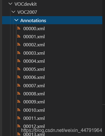
训练前将标签文件放在VOCdevkit文件夹下的VOC2007文件夹下的Annotation中。
训练前将图片文件放在VOCdevkit文件夹下的VOC2007文件夹下的JPEGImages中。

此时数据集的摆放已经结束。
二、数据集的处理
在完成数据集的摆放之后,我们需要对数据集进行下一步的处理,目的是获得训练用的2007_train.txt以及2007_val.txt,需要用到根目录下的voc_annotation.py。
voc_annotation.py里面有一些参数需要设置。
分别是annotation_mode、classes_path、trainval_percent、train_percent、VOCdevkit_path,第一次训练可以仅修改classes_path
'''
annotation_mode用于指定该文件运行时计算的内容
annotation_mode为0代表整个标签处理过程,包括获得VOCdevkit/VOC2007/ImageSets里面的txt以及训练用的2007_train.txt、2007_val.txt
annotation_mode为1代表获得VOCdevkit/VOC2007/ImageSets里面的txt
annotation_mode为2代表获得训练用的2007_train.txt、2007_val.txt
'''
annotation_mode     = 0
'''
必须要修改,用于生成2007_train.txt、2007_val.txt的目标信息
与训练和预测所用的classes_path一致即可
如果生成的2007_train.txt里面没有目标信息
那么就是因为classes没有设定正确
仅在annotation_mode为0和2的时候有效
'''
classes_path        = 'model_data/voc_classes.txt'
'''
trainval_percent用于指定(训练集+验证集)与测试集的比例,默认情况下 (训练集+验证集):测试集 = 9:1
train_percent用于指定(训练集+验证集)中训练集与验证集的比例,默认情况下 训练集:验证集 = 9:1
仅在annotation_mode为0和1的时候有效
'''
trainval_percent    = 0.9
train_percent       = 0.9
'''
指向VOC数据集所在的文件夹
默认指向根目录下的VOC数据集
'''
VOCdevkit_path  = 'VOCdevkit'
classes_path用于指向检测类别所对应的txt,以voc数据集为例,我们用的txt为:

训练自己的数据集时,可以自己建立一个cls_classes.txt,里面写自己所需要区分的类别。
三、开始网络训练
通过voc_annotation.py我们已经生成了2007_train.txt以及2007_val.txt,此时我们可以开始训练了。
训练的参数较多,大家可以在下载库后仔细看注释,其中最重要的部分依然是train.py里的classes_path。
classes_path用于指向检测类别所对应的txt,这个txt和voc_annotation.py里面的txt一样!训练自己的数据集必须要修改!

修改完classes_path后就可以运行train.py开始训练了,在训练多个epoch后,权值会生成在logs文件夹中。
其它参数的作用如下:
#------------------------------------------------------#
#   是否使用eager模式训练
#------------------------------------------------------#
eager = False
#------------------------------------------------------#
#   训练前一定要修改classes_path,使其对应自己的数据集
#------------------------------------------------------#
classes_path    = 'model_data/voc_classes.txt'
#----------------------------------------------------------------------------------------------------------------------------#
#   权值文件请看README,百度网盘下载。数据的预训练权重对不同数据集是通用的,因为特征是通用的。
#   预训练权重对于99%的情况都必须要用,不用的话权值太过随机,特征提取效果不明显,网络训练的结果也不会好。
#   训练自己的数据集时提示维度不匹配正常,预测的东西都不一样了自然维度不匹配
#
#   如果想要断点续练就将model_path设置成logs文件夹下已经训练的权值文件。
#   当model_path = ''的时候不加载整个模型的权值。
#
#   此处使用的是整个模型的权重,因此是在train.py进行加载的。
#   如果想要让模型从0开始训练,则设置model_path = '',下面的Freeze_Train = Fasle,此时从0开始训练,且没有冻结主干的过程。
#   一般来讲,从0开始训练效果会很差,因为权值太过随机,特征提取效果不明显。
#----------------------------------------------------------------------------------------------------------------------------#
model_path      = 'model_data/yolox_s.h5'
#------------------------------------------------------#
#   输入的shape大小,一定要是32的倍数
#------------------------------------------------------#
input_shape     = [640, 640]
#---------------------------------------------------------------------#
#   所使用的YoloX的版本。s、m、l、x
#---------------------------------------------------------------------#
phi             = 's'
#------------------------------------------------------------------------------------------------------------#
#   YoloX的tricks应用
#   mosaic 马赛克数据增强 True or False
#   YOLOX作者强调要在训练结束前的N个epoch关掉Mosaic。因为Mosaic生成的训练图片,远远脱离自然图片的真实分布。
#   并且Mosaic大量的crop操作会带来很多不准确的标注框,本代码自动会在前90%个epoch使用mosaic,后面不使用。
#   Cosine_scheduler 余弦退火学习率 True or False
#------------------------------------------------------------------------------------------------------------#
mosaic              = False
Cosine_scheduler    = False

#------------------------------------------------------#
#   训练分为两个阶段,分别是冻结阶段和解冻阶段。
#   显存不足与数据集大小无关,提示显存不足请调小batch_size。
#   受到BatchNorm层影响,batch_size最小为2,不能为1。
#------------------------------------------------------#
#------------------------------------------------------#
#   冻结阶段训练参数
#   此时模型的主干被冻结了,特征提取网络不发生改变
#   占用的显存较小,仅对网络进行微调
#------------------------------------------------------#
Init_Epoch          = 0
Freeze_Epoch        = 50
Freeze_batch_size   = 8
Freeze_lr           = 1e-3
#------------------------------------------------------#
#   解冻阶段训练参数
#   此时模型的主干不被冻结了,特征提取网络会发生改变
#   占用的显存较大,网络所有的参数都会发生改变
#------------------------------------------------------#
UnFreeze_Epoch      = 100
Unfreeze_batch_size = 4
Unfreeze_lr         = 1e-4
#------------------------------------------------------#
#   是否进行冻结训练,默认先冻结主干训练后解冻训练。
#------------------------------------------------------#
Freeze_Train        = True
#------------------------------------------------------#
#   用于设置是否使用多线程读取数据,0代表关闭多线程
#   开启后会加快数据读取速度,但是会占用更多内存
#   keras里开启多线程有些时候速度反而慢了许多
#   在IO为瓶颈的时候再开启多线程,即GPU运算速度远大于读取图片的速度。
#------------------------------------------------------#
num_workers         = 2
#------------------------------------------------------#
#   获得图片路径和标签
#------------------------------------------------------#
train_annotation_path   = '2007_train.txt'
val_annotation_path     = '2007_val.txt'
四、训练结果预测
训练结果预测需要用到两个文件,分别是yolo.py和predict.py。
我们首先需要去yolo.py里面修改model_path以及classes_path,这两个参数必须要修改。
model_path指向训练好的权值文件,在logs文件夹里。
classes_path指向检测类别所对应的txt。
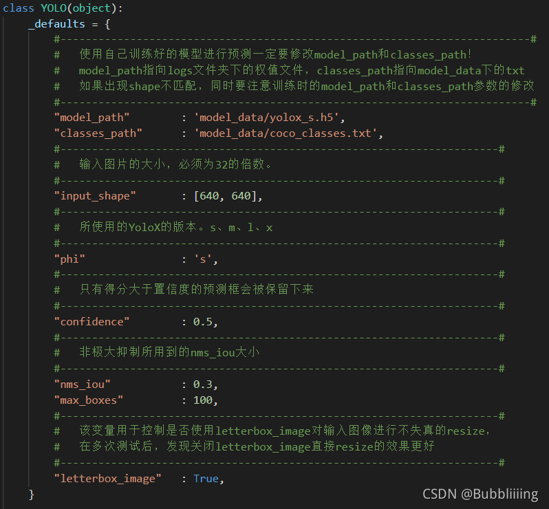
完成修改后就可以运行predict.py进行检测了。运行后输入图片路径即可检测。