1、sift特征原理的描述
1.1sift概述:
首先我了解到了兴趣点的概念,兴趣点是图像中明显区别于周围区域的地方,这些兴趣点对于光照、视角相当鲁棒,所以对于图像的兴趣点特征提取的好坏会直接影响到后续分类,识别的精准。而描述子就是对兴趣点提取特征的过程。sift是一种特征描述子。该描述子具有尺度不变性和光照不变性。
1.2sift特征检测的步骤:
sift特征检测有四个主要步骤:
1、尺度空间的极值检测:搜索所有尺度空间上的图像,通过高斯微分函数来识别潜在的对尺度和选择不变的兴趣点。
2、特征点定位:在每个候选的位置上,通过一个拟合精细模型来确定位置尺度,关键点的选取依据他们的稳定程度。
3、特征方向赋值:基于图像局部的梯度方向,分配给每个关键点位置一个或多个方向,后续的所有操作都是对于关键点的方向、尺度和位置进行变换,从而提供这些特征的不变性。
4、特征点描述:在每个特征点周围的邻域内,在选定的尺度上测量图像的局部梯度,这些梯度被变换成一种表示,这种表示允许比较大的局部形状的变换和光照变换。
2.1对sift特征检测的理解:
首先两张照片能够匹配上的前提是他们的 特征点的相似度比较高。
特征点的检出主要用了DoG,就是把图像做不同的高斯模糊,平滑的区域或点肯定变化不是很大,而纹理复杂的地方比如边缘、点、角之类的区域变化很大,像这样变化很大的点就是特征点,特征点描述就是简单的HOG,就是以检出的特征点为中心选16*16的区域作为local patch,这个区域又可以均分为4*4个子区域,每个子区域中各个像素的梯度都可以分到8个bin里面,这样子就得到了4*4*8=128维度的特征向量。当一个点如果在DoG空间本层以及上下两层的26个领域中是最大值和最小值时,就认为该点是图像在该尺度下的一个特征点。

2、sift和Harris特征匹配处理图片的对比
以下是分别用sift和harris对同一张图片进行特征提取实验的代码:
# -*- coding: utf-8 -*-
from PIL import Image
from pylab import *
from PCV.localdescriptors import sift
from PCV.localdescriptors import harris

# 添加中文字体支持
from matplotlib.font_manager import FontProperties
font = FontProperties(fname=r"c:\windows\fonts\SimSun.ttc", size=14)

imname = 'D:/pythonxy/PCV-book-data/data/panoimage/a.jpg'
im = array(Image.open(imname).convert('L'))
sift.process_image(imname, 'empire.sift')
l1, d1 = sift.read_features_from_file('empire.sift')

figure()
gray()
subplot(131)
sift.plot_features(im, l1, circle=False)
title(u'SIFT特征',fontproperties=font)
subplot(132)
sift.plot_features(im, l1, circle=True)
title(u'用圆圈表示SIFT特征尺度',fontproperties=font)

# 检测harris角点
harrisim = harris.compute_harris_response(im)

subplot(133)
filtered_coords = harris.get_harris_points(harrisim, 6, 0.1)
imshow(im)
plot([p[1] for p in filtered_coords], [p[0] for p in filtered_coords], '*')
axis('off')
title(u'Harris角点',fontproperties=font)

show()
以下是运行的结果图:
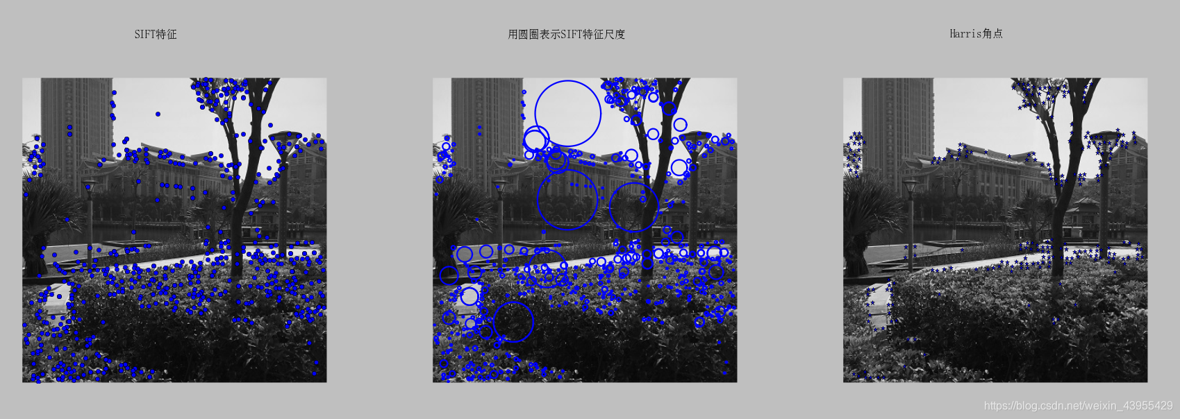
从图中可以看出,两个算法所选择特征点的位置不同。
Harris算法在图像变换次数较多的情况下相比于sift算法提取特征点坐标偏移量相对较小。
3、使用sift对两张图片初步匹配结果
以下是运行的代码:
*sift.py
from PIL import Image
import os
from numpy import *
from pylab import *


def process_image(imagename,resultname,params="--edge-thresh 10 --peak-thresh 5"):
    """ process an image and save the results in a file"""
    path = os.path.abspath(os.path.join(os.path.dirname("__file__"),os.path.pardir))
    path = path+"\\utils\\win32vlfeat\\sift.exe "
    if imagename[-3:] != 'pgm':
	    #create a pgm file
		 im = Image.open(imagename).convert('L')
		 im.save('tmp.pgm')
		 imagename = 'tmp.pgm'
    cmmd = str("D:\pythonxy\win64vlfeat\sift.exe "+imagename+" --output="+resultname+
				" "+params)
    os.system(cmmd)
    print 'processed', imagename, 'to', resultname


def read_features_from_file(filename):
	""" read feature properties and return in matrix form"""
	f = loadtxt(filename)
	return f[:,:4],f[:,4:] # feature locations, descriptors


def write_features_to_file(filename,locs,desc):
	""" save feature location and descriptor to file"""
	savetxt(filename,hstack((locs,desc)))


def plot_features(im,locs,circle=False):
	""" show image with features. input: im (image as array),
		locs (row, col, scale, orientation of each feature) """

	def draw_circle(c,r):
		t = arange(0,1.01,.01)*2*pi
		x = r*cos(t) + c[0]
		y = r*sin(t) + c[1]
		plot(x,y,'b',linewidth=2)

	imshow(im)
	if circle:
		[draw_circle([p[0],p[1]],p[2]) for p in locs]
	else:
		plot(locs[:,0],locs[:,1],'ob')
	axis('off')


def match(desc1,desc2):
	""" for each descriptor in the first image,
		select its match in the second image.
		input: desc1 (descriptors for the first image),
		desc2 (same for second image). """

	desc1 = array([d/linalg.norm(d) for d in desc1])
	desc2 = array([d/linalg.norm(d) for d in desc2])

	dist_ratio = 0.6
	desc1_size = desc1.shape

	matchscores = zeros((desc1_size[0],1))
	desc2t = desc2.T #precompute matrix transpose
	for i in range(desc1_size[0]):
		dotprods = dot(desc1[i,:],desc2t) #vector of dot products
		dotprods = 0.9999*dotprods
		#inverse cosine and sort, return index for features in second image
		indx = argsort(arccos(dotprods))

		#check if nearest neighbor has angle less than dist_ratio times 2nd
		if arccos(dotprods)[indx[0]] < dist_ratio * arccos(dotprods)[indx[1]]:
			matchscores[i] = int(indx[0])

	return matchscores


def appendimages(im1,im2):
	""" return a new image that appends the two images side-by-side."""

	#select the image with the fewest rows and fill in enough empty rows
	rows1 = im1.shape[0]
	rows2 = im2.shape[0]

	if rows1 < rows2:
		im1 = concatenate((im1,zeros((rows2-rows1,im1.shape[1]))), axis=0)
	elif rows1 > rows2:
		im2 = concatenate((im2,zeros((rows1-rows2,im2.shape[1]))), axis=0)
	#if none of these cases they are equal, no filling needed.

	return concatenate((im1,im2), axis=1)


def plot_matches(im1,im2,locs1,locs2,matchscores,show_below=True):
	""" show a figure with lines joining the accepted matches
		input: im1,im2 (images as arrays), locs1,locs2 (location of features),
		matchscores (as output from 'match'), show_below (if images should be shown below). """

	im3 = appendimages(im1,im2)
	if show_below:
		im3 = vstack((im3,im3))

	# show image
	imshow(im3)

	# draw lines for matches
	cols1 = im1.shape[1]
	for i in range(len(matchscores)):
		if matchscores[i] > 0:
			plot([locs1[i,0], locs2[matchscores[i,0],0]+cols1], [locs1[i,1], locs2[matchscores[i,0],1]], 'c')
	axis('off')


def match_twosided(desc1,desc2):
	""" two-sided symmetric version of match(). """

	matches_12 = match(desc1,desc2)
	matches_21 = match(desc2,desc1)

	ndx_12 = matches_12.nonzero()[0]

	#remove matches that are not symmetric
	for n in ndx_12:
		if matches_21[int(matches_12[n])] != n:
			matches_12[n] = 0

	return matches_12


if __name__ == "__main__":

	process_image('box.pgm','tmp.sift')
	l,d = read_features_from_file('tmp.sift')

	im = array(Image.open('box.pgm'))
	figure()
	plot_features(im,l,True)
	gray()

	process_image('scene.pgm','tmp2.sift')
	l2,d2 = read_features_from_file('tmp2.sift')
	im2 = array(Image.open('scene.pgm'))

	m = match_twosided(d,d2)
	figure()
	plot_matches(im,im2,l,l2,m)

	gray()
	show()
*sift_match.py
from PIL import Image
from pylab import *
import sys
from PCV.localdescriptors import sift


if len(sys.argv) >= 3:
  im1f, im2f = sys.argv[1], sys.argv[2]
else:
  im1f = 'D:/pythonxy/PCV-book-data/data/panoimage/d.jpg'
  im2f = 'D:/pythonxy/PCV-book-data/data/panoimage/e.jpg'
im1 = array(Image.open(im1f))
im2 = array(Image.open(im2f))

sift.process_image(im1f, 'out_sift_3.txt')
l1, d1 = sift.read_features_from_file('out_sift_3.txt')
figure()
gray()
subplot(121)
sift.plot_features(im1, l1, circle=False)

sift.process_image(im2f, 'out_sift_4.txt')
l2, d2 = sift.read_features_from_file('out_sift_4.txt')
subplot(122)
sift.plot_features(im2, l2, circle=False)

#matches = sift.match(d1, d2)
matches = sift.match_twosided(d1, d2)
print '{} matches'.format(len(matches.nonzero()[0]))

figure()
gray()
sift.plot_matches(im1, im2, l1, l2, matches, show_below=True)
show()
以下是运行的结果图:
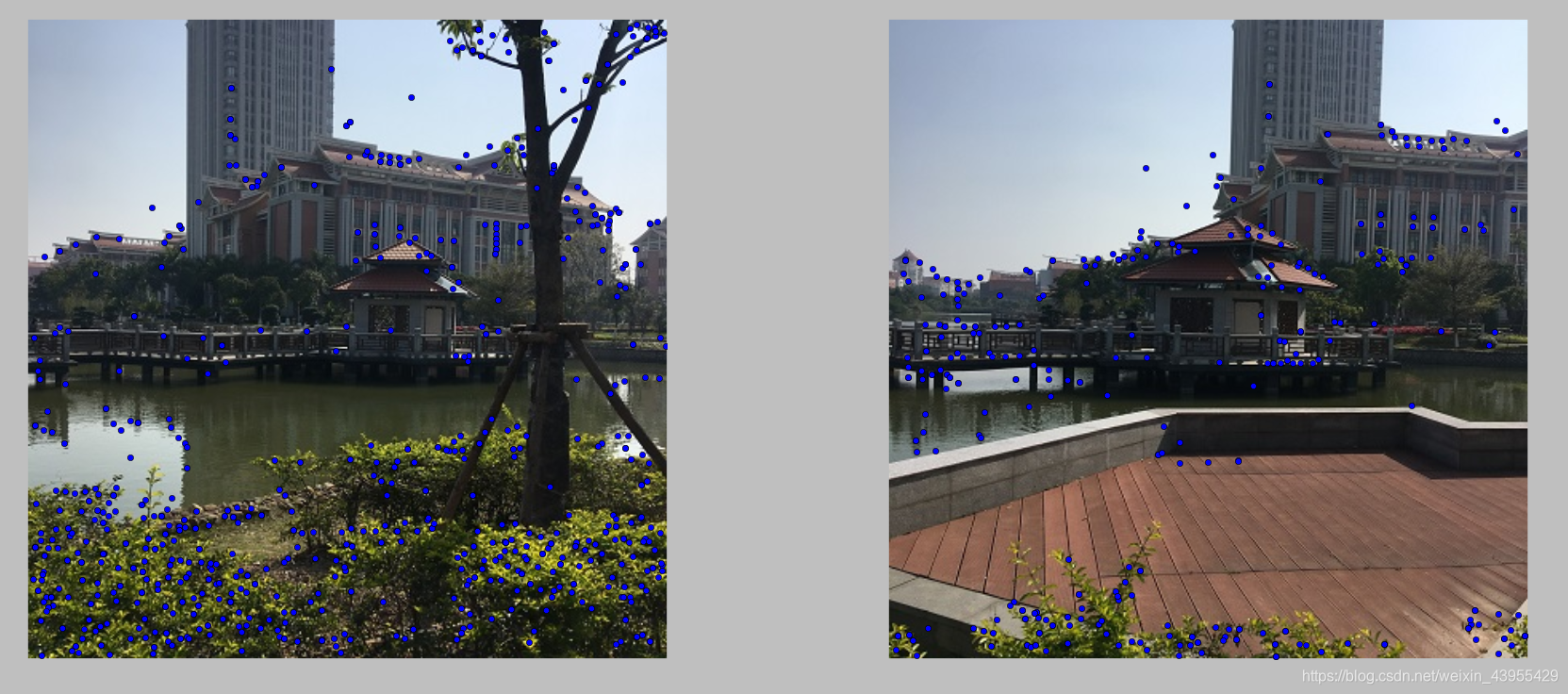
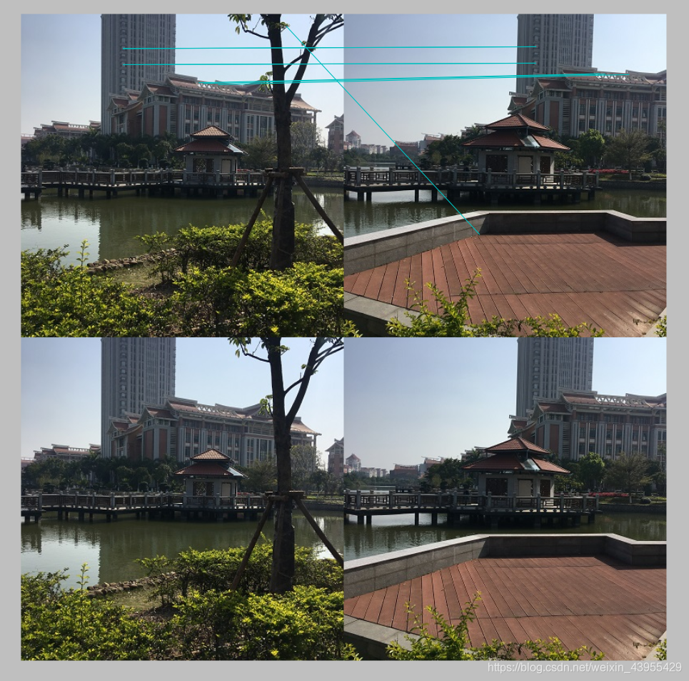
以上是进行了描述子匹配的结果图。可以看出图一对两张图片进行了特征提取,图二对两张图片进行了匹配,通过match_twosided()函数返回的特征点匹配情况。对于将一幅图像中的特征匹配到另一幅图像的特征,一种稳健的准则是使用这两个特征距离和两个最匹配特征距离的比率。相比于图像中的其他特征,该准则保证能够找到足够相似的唯一特征。使用这个方法可以使错误的匹配数降低。
4、使用集美大学不同视角拍摄的图片做地理标记
以下是运行的代码:
# -*- coding: utf-8 -*-
from pylab import *
from PIL import Image
from PCV.localdescriptors import sift
from PCV.tools import imtools
import pydot
import os

""" This is the example graph illustration of matching images from Figure 2-10.
To download the images, see ch2_download_panoramio.py."""

#download_path = "panoimages"  # set this to the path where you downloaded the panoramio images
#path = "/FULLPATH/panoimages/"  # path to save thumbnails (pydot needs the full system path)

download_path = "D:/pythonxy/PCV-book-data/data/panoimages"  # set this to the path where you downloaded the panoramio images
path = "D:/pythonxy/PCV-book-data/data/panoimages/"  # path to save thumbnails (pydot needs the full system path)

# list of downloaded filenames
imlist = imtools.get_imlist(download_path)
nbr_images = len(imlist)

# extract features
featlist = [imname[:-3] + 'sift' for imname in imlist]
for i, imname in enumerate(imlist):
    sift.process_image(imname, featlist[i])

matchscores = zeros((nbr_images, nbr_images))

for i in range(nbr_images):
    for j in range(i, nbr_images):  # only compute upper triangle
        print 'comparing ', imlist[i], imlist[j]
        l1, d1 = sift.read_features_from_file(featlist[i])
        l2, d2 = sift.read_features_from_file(featlist[j])
        matches = sift.match_twosided(d1, d2)
        nbr_matches = sum(matches > 0)
        print 'number of matches = ', nbr_matches
        matchscores[i, j] = nbr_matches
    print "The match scores is: %d", matchscores

#np.savetxt(("../data/panoimages/panoramio_matches.txt",matchscores)

# copy values
for i in range(nbr_images):
    for j in range(i + 1, nbr_images):  # no need to copy diagonal
        matchscores[j, i] = matchscores[i, j]

threshold = 2  # min number of matches needed to create link

g = pydot.Dot(graph_type='graph')  # don't want the default directed graph

for i in range(nbr_images):
    for j in range(i + 1, nbr_images):
        if matchscores[i, j] > threshold:
            # first image in pair
            im = Image.open(imlist[i])
            im.thumbnail((100, 100))
            filename = path + str(i) + '.png'
            im.save(filename)  # need temporary files of the right size
            g.add_node(pydot.Node(str(i), fontcolor='transparent', shape='rectangle', image=filename))

            # second image in pair
            im = Image.open(imlist[j])
            im.thumbnail((100, 100))
            filename = path + str(j) + '.png'
            im.save(filename)  # need temporary files of the right size
            g.add_node(pydot.Node(str(j), fontcolor='transparent', shape='rectangle', image=filename))

            g.add_edge(pydot.Edge(str(i), str(j)))
g.write_png('whitehouse.png')
以下是运行的结果图:
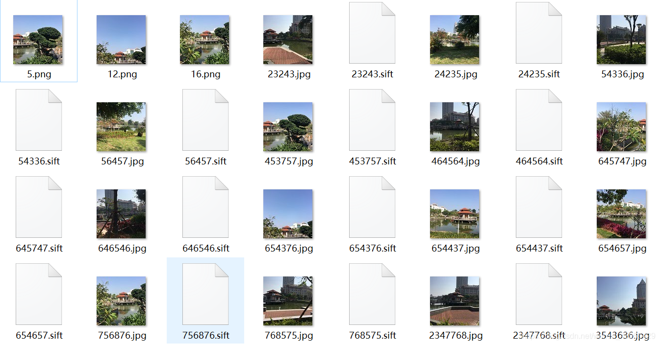
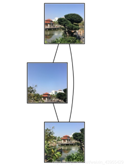
可能因为图片中相似的特征物不是很明显,于是我换了一组素材再测试之后的结果如下:
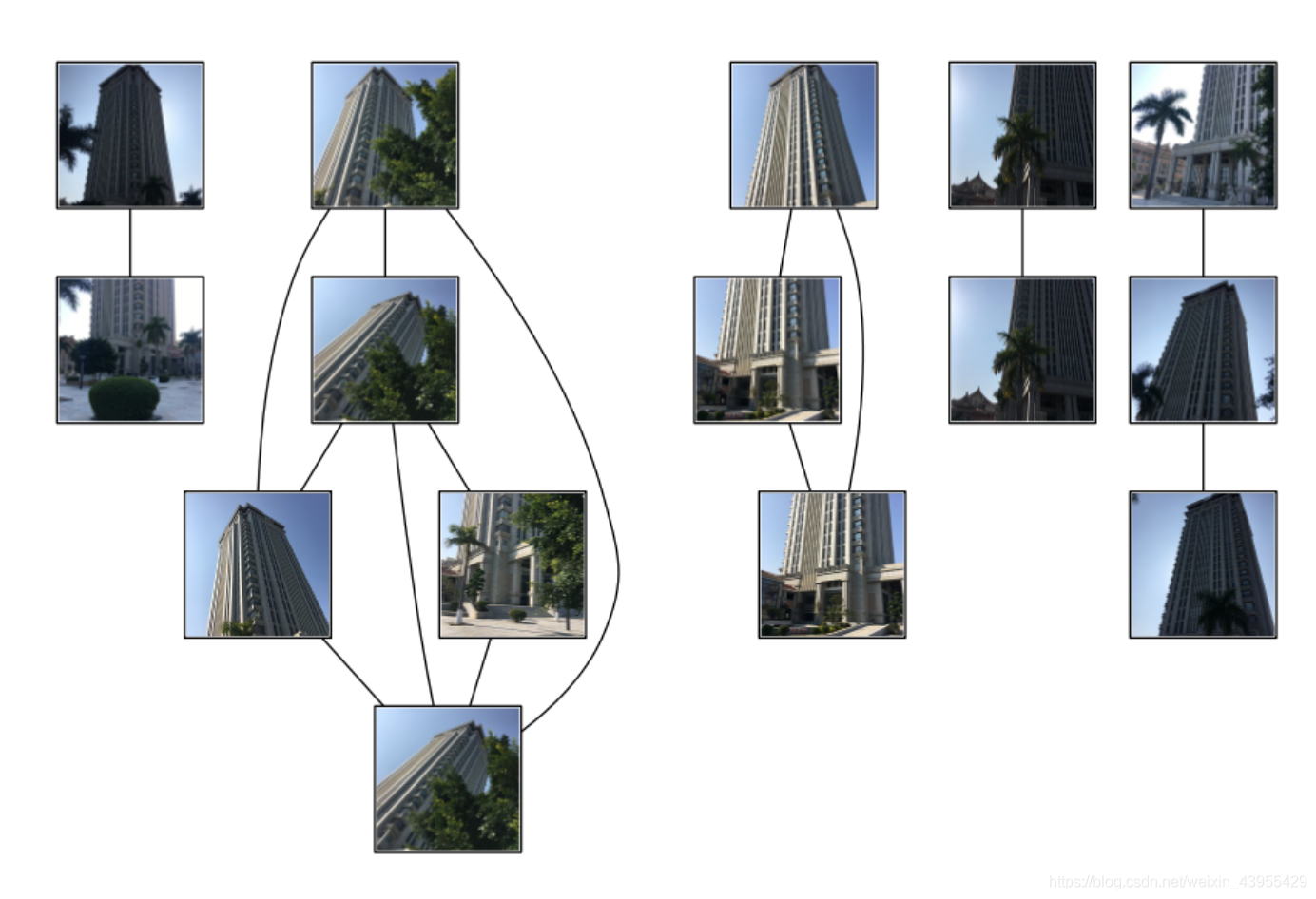
以上结果首先经过局部描述子匹配,将每对图像间的匹配特征数保存在matchscores数组中。因为该“距离矢量”是对称的,所以我们可以不在代码的最后部分复制数值来将matchscores矩阵填充完整;填充完整后的matchscores矩阵只是看起来更好。然后使用该matchscores矩阵作为图像间简单的距离度量方式。
然后进行可视化连接的图像,通过图像间是否具有匹配的局部描述子来定义图像间的连接,然后可视化这些连接情况。为了完成可视化,我们可以在图中显示这些图像,图的边代表连接。其中会使用到pydot工具包。然后为了创建显示可能图像组的图,如果匹配的数目高于一个阈值,我们使用边来连接相应的图像节点。为了得到图中的图像,使用图像的全路径。为了使图像看起来更好以及运行速度更快,我将图像都调整为200*200像素。
