作业内容：

Q1: k-Nearest Neighbor classifier (20 points)
Q2: Training a Support Vector Machine (25 points)
Q3: Implement a Softmax classifier (20 points)
Q4: Two-Layer Neural Network (25 points)
Q5: Higher Level Representations: Image Features (10 points)

Q1：k-Nearest Neighbor classifier

完成一个KNN classifier 总共需要做两件事情：
第一件事情是将所有的training data读入
第二件事情是给定testing image 然后让其与所有的training data对比，然后将这幅图像的标签定位k个最近的image的标签。
所以，KNN可以说成是不需要训练时间的，但测试时间往往开销很大。

下面我将一步步解释cs231n assignment #1 中knn的代码

Step 1

# Run some setup code for this notebook.

import random
import numpy as np
from cs231n.data_utils import load_CIFAR10
import matplotlib.pyplot as plt

# This is a bit of magic to make matplotlib figures appear inline in the notebook
# rather than in a new window.
%matplotlib inline
plt.rcParams['figure.figsize'] = (10.0, 8.0) # set default size of plots
plt.rcParams['image.interpolation'] = 'nearest'
plt.rcParams['image.cmap'] = 'gray'

# Some more magic so that the notebook will reload external python modules;
# see http://stackoverflow.com/questions/1907993/autoreload-of-modules-in-ipython
%load_ext autoreload
%autoreload 2

在这里为load_CIFAR10模块的作用是加载数据集，此函数的返回值是return Xtr, Ytr, Xte, Yte
autoreload 2：自动重载%aimport排除的模块之外的所有模块，因为后面要求你修改.py文件里面的内容有了这个autoreeload之后，修改之后就会重新加载，在这里我们不深究是什么意思。

Step 2

# Load the raw CIFAR-10 data.
cifar10_dir = 'cs231n/datasets/cifar-10-batches-py'

# Cleaning up variables to prevent loading data multiple times (which may cause memory issue)
try:
   del X_train, y_train
   del X_test, y_test
   print('Clear previously loaded data.')
except:
   pass
# 这里的try except是为了防止多次loading
X_train, y_train, X_test, y_test = load_CIFAR10(cifar10_dir)

# As a sanity check, we print out the size of the training and test data.
print('Training data shape: ', X_train.shape)
print('Training labels shape: ', y_train.shape)
print('Test data shape: ', X_test.shape)
print('Test labels shape: ', y_test.shape)

数据集已经载入成功了：

Training data shape:  (50000, 32, 32, 3)
Training labels shape:  (50000,)
Test data shape:  (10000, 32, 32, 3)
Test labels shape:  (10000,)

Step 3

# Visualize some examples from the dataset.
# We show a few examples of training images from each class.
classes = ['plane', 'car', 'bird', 'cat', 'deer', 'dog', 'frog', 'horse', 'ship', 'truck']
num_classes = len(classes)
samples_per_class = 7
for y, cls in enumerate(classes):
    idxs = np.flatnonzero(y_train == y)
    # np.flatnonzero()函数输入一个矩阵，返回扁平化后矩阵中非零元素的位置（index）
    idxs = np.random.choice(idxs, samples_per_class, replace=False)
    for i, idx in enumerate(idxs):
        plt_idx = i * num_classes + y + 1
        plt.subplot(samples_per_class, num_classes, plt_idx)
        plt.imshow(X_train[idx].astype('uint8'))
        plt.axis('off')
        if i == 0:
            plt.title(cls)
plt.show()

在这里插入图片描述

Step 4

# Subsample the data for more efficient code execution in this exercise
num_training = 5000
mask = list(range(num_training))
X_train = X_train[mask]
y_train = y_train[mask]

num_test = 500
mask = list(range(num_test))
X_test = X_test[mask]
y_test = y_test[mask]

# Reshape the image data into rows
X_train = np.reshape(X_train, (X_train.shape[0], -1))
X_test = np.reshape(X_test, (X_test.shape[0], -1))
print(X_train.shape, X_test.shape)

这里的Subsample并不是下采样的意思，只是因为原来的数据集的图片数量很多，在我们这个小小的demo中只需要取少量来演示就行。所以就在原来50000张training中选取5000张，10000张testing testing data中选取500张作为我们demo的data set

(5000, 3072) (500, 3072)

Step 5

from cs231n.classifiers import KNearestNeighbor

# Create a kNN classifier instance. 
# Remember that training a kNN classifier is a noop(空操作): 
# the Classifier simply remembers the data and does no further processing 
classifier = KNearestNeighbor()
classifier.train(X_train, y_train)

这是原文，如果你不想看英文，下面有翻译：
We would now like to classify the test data with the kNN classifier. Recall that we can break down this process into two steps:

First we must compute the distances between all test examples and all train examples.
Given these distances, for each test example we find the k nearest examples and have them vote for the label

Lets begin with computing the distance matrix between all training and test examples. For example, if there are Ntr training examples and Nte test examples, this stage should result in a Nte x Ntr matrix where each element (i,j) is the distance between the i-th test and j-th train example.

Note: For the three distance computations that we require you to implement in this notebook, you may not use the np.linalg.norm() function that numpy provides.

First, open cs231n/classifiers/k_nearest_neighbor.py and implement the function compute_distances_two_loops that uses a (very inefficient) double loop over all pairs of (test, train) examples and computes the distance matrix one element at a time.

翻译如下：
先来对test data 进行分类，回想以下我们之前所说的，要实现分类我们应该：

计算test data中每一张图片于training data中所有图片的distances
更具K个最近的图片(distances 最小) 投票选出这张图片的lable

让我们从计算distance matrix 开始，假如你有N个training examples 和 M个testing examples那么我们需要做的就是计算出M x N 的矩阵，每一个矩阵中的元素element (i,j)都是一张testing image 到一张training image 的距离。

Note:每一个计算距离的算法都要求动手实现，并且还不能用np.linalg.norm()这些numpy
已经提供的函数，所以得自己写函数（斯坦福果然要求严格）

首先，打开cs231n/classifiers/k_nearest_neighbor.py并实现compute_distances_two_loops函数，该函数在所有（测试、训练）示例上使用非常低效的双循环，并一次计算一个矩阵中的元素。

打开文件之后写下计算L2距离的公式：dists[i, j] = np.sqrt(np.sum(np.square(X[i] - self.X_train[j])))虽然这个公式的计算效率很低但是作为初学者，我们可以不太考虑效率的问题。

  def compute_distances_two_loops(self, X):
        """
        Compute the distance between each test point in X and each training point
        in self.X_train using a nested loop（嵌套循环） over both the training data and the
        test data.

        Inputs:
        - X: A numpy array of shape (num_test, D) containing test data.

        Returns:
        - dists: A numpy array of shape (num_test, num_train) where dists[i, j]
          is the Euclidean distance between the ith test point and the jth training
          point.
        """
        num_test = X.shape[0]
        num_train = self.X_train.shape[0]
        dists = np.zeros((num_test, num_train))
        for i in range(num_test):
            for j in range(num_train):
                #####################################################################
                # TODO:                                                             #
                # Compute the l2 distance between the ith test point and the jth    #
                # training point, and store the result in dists[i, j]. You should   #
                # not use a loop over dimension, nor use np.linalg.norm().          #
                #####################################################################
                # *****START OF YOUR CODE (DO NOT DELETE/MODIFY THIS LINE)*****
                dists[i, j] = np.sqrt(np.sum((X[i]-self.X_train[j])**2))
                pass

                # *****END OF YOUR CODE (DO NOT DELETE/MODIFY THIS LINE)*****
        return dists

Step 6

# Open cs231n/classifiers/k_nearest_neighbor.py and implement
# compute_distances_two_loops.

# Test your implementation:
dists = classifier.compute_distances_two_loops(X_test)
print(dists.shape)

(500, 5000)

# We can visualize the distance matrix: each row is a single test example and
# its distances to training examples
plt.imshow(dists, interpolation='none')
plt.show()

如果你显示的是全黑色就说明compute_distances_two_loops函数没有写或者是写错了
在这里插入图片描述
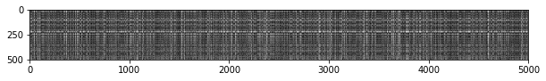
x轴是traning data ，y轴是testing data ， black indicates low distances while white indicates high distances（黑色表示距离很小，白色表示距离很大，像素值越大越亮嘛）

Inline Question 1

Notice the structured patterns in the distance matrix, where some rows or columns are visible brighter. (Note that with the default color scheme black indicates low distances while white indicates high distances.)

What in the data is the cause behind the distinctly bright rows?
What causes the columns?

$\color{blue}{\textit Your Answer:}$ 1.两张图片的L2距离越小，既像素值越低，所以图片上会显示出黑色，反之则为白色（由于distance>255所以我怀疑在可视化的时候有把distance的值约束在0～255之间）2.第二个问题我不知道在问什么，希望大佬指点

在下面这一步之前你得到k_nearest_neighbor.py文件中把剩余部分补充完整

    def predict_labels(self, dists, k=1):
        """
        Given a matrix of distances between test points and training points,
        predict a label for each test point.

        Inputs:
        - dists: A numpy array of shape (num_test, num_train) where dists[i, j]
          gives the distance betwen the ith test point and the jth training point.

        Returns:
        - y: A numpy array of shape (num_test,) containing predicted labels for the
          test data, where y[i] is the predicted label for the test point X[i].
        """
        num_test = dists.shape[0]
        y_pred = np.zeros(num_test)
        for i in range(num_test):
            # A list of length k storing the labels of the k nearest neighbors to
            # the ith test point.
            closest_y = []
            #########################################################################
            # TODO:                                                                 #
            # Use the distance matrix to find the k nearest neighbors of the ith    #
            # testing point, and use self.y_train to find the labels of these       #
            # neighbors. Store these labels in closest_y.                           #
            # Hint: Look up the function numpy.argsort.                             #
            # argsort函数返回的是数组值从小到大的索引值
            #########################################################################
            # *****START OF YOUR CODE (DO NOT DELETE/MODIFY THIS LINE)*****
            closest_y = self.y_train[np.argsort(dists[i])[:k]]
            pass

            # *****END OF YOUR CODE (DO NOT DELETE/MODIFY THIS LINE)*****
            #########################################################################
            # TODO:                                                                 #
            # Now that you have found the labels of the k nearest neighbors, you    #
            # need to find the most common label in the list closest_y of labels.   #
            # Store this label in y_pred[i]. Break ties by choosing the smaller     #
            # label.                                                                #
            #########################################################################
            # *****START OF YOUR CODE (DO NOT DELETE/MODIFY THIS LINE)*****
            timeLabel = sorted([(np.sum(closest_y == y_), y_) for y_ in set(closest_y)])[-1]
            y_pred[i] = timeLabel[1]
            pass

            # *****END OF YOUR CODE (DO NOT DELETE/MODIFY THIS LINE)*****

        return y_pred

Step 7

# Now implement the function predict_labels and run the code below:
# We use k = 1 (which is Nearest Neighbor).
y_test_pred = classifier.predict_labels(dists, k=1)

# Compute and print the fraction（小部分） of correctly predicted examples
num_correct = np.sum(y_test_pred == y_test)
accuracy = float(num_correct) / num_test
print('Got %d / %d correct => accuracy: %f' % (num_correct, num_test, accuracy))

可以见得，当k=1的时候，准确率是相当的低:
Got 137 / 500 correct => accuracy: 0.274000

所以现在的想法是通过提升K来提高准确：

y_test_pred = classifier.predict_labels(dists, k=5)
num_correct = np.sum(y_test_pred == y_test)
accuracy = float(num_correct) / num_test
print('Got %d / %d correct => accuracy: %f' % (num_correct, num_test, accuracy))

Got 143 / 500 correct => accuracy: 0.286000
效果确实好了一点。

Inline Question 2

We can also use other distance metrics such as L1 distance.
For pixel values $p_{ij}^{(k)}$ at location $(i,j)$ of some image $I_k$ ,

the mean $\mu$ across all pixels over all images is $\mu=\frac{1}{nhw}\sum_{k=1}^n\sum_{i=1}^{h}\sum_{j=1}^{w}p_{ij}^{(k)}$
And the pixel-wise mean $\mu_{ij}$ across all images is
$\mu_{ij}=\frac{1}{n}\sum_{k=1}^np_{ij}^{(k)}.$
The general standard deviation $\sigma$ and pixel-wise standard deviation $\sigma_{ij}$ is defined similarly.

Which of the following preprocessing steps will not change the performance of a Nearest Neighbor classifier that uses L1 distance? Select all that apply.

Subtracting the mean $\mu$ ( $\tilde{p}_{ij}^{(k)}=p_{ij}^{(k)}-\mu$ .)
Subtracting the per pixel mean $\mu_{ij}$ ( $\tilde{p}_{ij}^{(k)}=p_{ij}^{(k)}-\mu_{ij}$ .)
Subtracting the mean $\mu$ and dividing by the standard deviation $\sigma$ .
Subtracting the pixel-wise mean $\mu_{ij}$ and dividing by the pixel-wise standard deviation $\sigma_{ij}$ .
Rotating the coordinate axes of the data.

$\color{blue}{\textit Your Answer:}$1&3&5 will not change.

$\color{blue}{\textit Your Explanation:}$ 对于给定的数据集来说，他们的mean和per pixel 都是常数，在计算距离相减的时候都会被抵消掉，然而当mean 除去一个标准差后的距离应该等于真正的L1 distance 乘以标准差，对于旋转数据的坐标轴，每张图片的像素和并不会改变，所以L1 distance也就不会改变

在这之前我们又要打开cs231n/classifiers/k_nearest_neighbor.py并补充compute_distances_one_loops函数
这个函数相比于compute_distances_two_loops将一个遍历training data 的循环用矩阵来实现，这样可以起到加速计算的作用，，self.X_train的shape为(5000, 3072)，循环一般都是比较好时间的，所以在我们的程序中应该尽量避免使用循环。

   def compute_distances_one_loop(self, X):
        """
        Compute the distance between each test point in X and each training point
        in self.X_train using a single loop over the test data.

        Input / Output: Same as compute_distances_two_loops
        """
        num_test = X.shape[0]
        num_train = self.X_train.shape[0]
        dists = np.zeros((num_test, num_train))
        for i in range(num_test):
            #######################################################################
            # TODO:                                                               #
            # Compute the l2 distance between the ith test point and all training #
            # points, and store the result in dists[i, :].                        #
            # Do not use np.linalg.norm().                                        #
            #######################################################################
            # *****START OF YOUR CODE (DO NOT DELETE/MODIFY THIS LINE)*****
            dists[i] = np.sqrt(np.sum(np.square(self.X_train - X[i]), axis=1))
            # 这里你会注意到self.X—_train的shape为(5000,3072)而X的shape为(500,3072)所以X[i]
            # 是一个向量,我对这样的矩阵减法有些疑惑,所以做了如下实验(往下翻)
            pass

            # *****END OF YOUR CODE (DO NOT DELETE/MODIFY THIS LINE)*****
        print(self.X_train.shape)
        print(X.shape)
        return dists

(3，3)matrix- (1,3)的matrix:

>>> y=np.array([1,2,3])
>>> x
array([[1, 2, 3],
       [4, 5, 6],
       [7, 8, 9]])
>>> y
array([1, 2, 3])
>>> x-y
array([[0, 0, 0],
       [3, 3, 3],
       [6, 6, 6]])
>>> y-x
array([[ 0,  0,  0],
       [-3, -3, -3],
       [-6, -6, -6]])

Step 8

# Now lets speed up distance matrix computation by using partial vectorization
# with one loop. Implement the function compute_distances_one_loop and run the
# code below:
dists_one = classifier.compute_distances_one_loop(X_test)

# To ensure that our vectorized implementation is correct, we make sure that it
# agrees with the naive implementation. There are many ways to decide whether
# two matrices are similar; one of the simplest is the Frobenius norm. In case
# you haven't seen it before, the Frobenius norm of two matrices is the square
# root of the squared sum of differences of all elements; in other words, reshape
# the matrices into vectors and compute the Euclidean distance between them.
difference = np.linalg.norm(dists - dists_one, ord='fro')
print('One loop difference was: %f' % (difference, ))
if difference < 0.001:
    print('Good! The distance matrices are the same')
else:
    print('Uh-oh! The distance matrices are different')

output:

One loop difference was: 0.000000
Good! The distance matrices are the same

在这之前我们又要打开cs231n/classifiers/k_nearest_neighbor.py并补充compute_distances_no_loops函数

   def compute_distances_no_loops(self, X):
        """
        Compute the distance between each test point in X and each training point
        in self.X_train using no explicit loops.

        Input / Output: Same as compute_distances_two_loops
        """
        num_test = X.shape[0]
        num_train = self.X_train.shape[0]
        dists = np.zeros((num_test, num_train))
        #########################################################################
        # TODO:                                                                 #
        # Compute the l2 distance between all test points and all training      #
        # points without using any explicit loops, and store the result in      #
        # dists.                                                                #
        #                                                                       #
        # You should implement this function using only basic array operations; #
        # in particular you should not use functions from scipy,                #
        # nor use np.linalg.norm().                                             #
        #                                                                       #
        # HINT: Try to formulate the l2 distance using matrix multiplication    #
        #       and two broadcast sums.                                         #
        #########################################################################
        # *****START OF YOUR CODE (DO NOT DELETE/MODIFY THIS LINE)*****
        # 在这里将L2distans 公式展开计算先分别计算两个矩阵的平方然后减去2倍的两个矩阵的和就得到了最终的distance
        dists += np.sum(self.X_train ** 2, axis=1).reshape(1, num_train)  # 这里其实利用了broadcast
        dists += np.sum(X ** 2, axis=1).reshape(num_test, 1)
        dists -= 2 * np.dot(X, self.X_train.T)  # np.dot(a,b)可以对两个矩阵求乘积，要求a的第二维与b的第一维长度一致
        dists = np.sqrt(dists)
        pass

        # *****END OF YOUR CODE (DO NOT DELETE/MODIFY THIS LINE)*****
        return dists

Step 9

# Now implement the fully vectorized version inside compute_distances_no_loops
# and run the code
dists_two = classifier.compute_distances_no_loops(X_test)

# check that the distance matrix agrees with the one we computed before:
difference = np.linalg.norm(dists - dists_two, ord='fro')
print('No loop difference was: %f' % (difference, ))
if difference < 0.001:
    print('Good! The distance matrices are the same')
else:
    print('Uh-oh! The distance matrices are different')

output：

No loop difference was: 0.000000
Good! The distance matrices are the same

Step 10

# Let's compare how fast the implementations are
def time_function(f, *args):
    """
    Call a function f with args and return the time (in seconds) that it took to execute.
    """
    import time
    tic = time.time()
    f(*args)
    toc = time.time()
    return toc - tic

two_loop_time = time_function(classifier.compute_distances_two_loops, X_test)
print('Two loop version took %f seconds' % two_loop_time)

one_loop_time = time_function(classifier.compute_distances_one_loop, X_test)
print('One loop version took %f seconds' % one_loop_time)

no_loop_time = time_function(classifier.compute_distances_no_loops, X_test)
print('No loop version took %f seconds' % no_loop_time)

# You should see significantly faster performance with the fully vectorized implementation!

# NOTE: depending on what machine you're using, 
# you might not see a speedup when you go from two loops to one loop, 
# and might even see a slow-down.

Step 11 Cross-validation

num_folds = 5
k_choices = [1, 3, 5, 8, 10, 12, 15, 20, 50, 100]

X_train_folds = []
y_train_folds = []
################################################################################
# TODO:                                                                        #
# Split up the training data into folds. After splitting, X_train_folds and    #
# y_train_folds should each be lists of length num_folds, where                #
# y_train_folds[i] is the label vector for the points in X_train_folds[i].     #
# Hint: Look up the numpy array_split function. ??lavel vector is what？？？    #
################################################################################
# *****START OF YOUR CODE (DO NOT DELETE/MODIFY THIS LINE)*****
# OK 上面的这个问题我已经解决了，label vector的意思就是5000张图片的标签，它的目的是知道你每个fold
# 里面的图片是原来5000张中的哪一张,下面两行代码的意思就是我不仅要把5000张图片的分成fold还要将他们的
# 标签分成几个fold
X_train_folds = np.array_split(X_train, num_folds)
Y_train_folds = np.array_split(y_train, num_folds)

pass

# *****END OF YOUR CODE (DO NOT DELETE/MODIFY THIS LINE)*****

# A dictionary holding the accuracies for different values of k that we find
# when running cross-validation. After running cross-validation,
# k_to_accuracies[k] should be a list of length num_folds giving the different
# accuracy values that we found when using that value of k.
k_to_accuracies = {}


################################################################################
# TODO:                                                                        #
# Perform k-fold cross validation to find the best value of k. For each        #
# possible value of k, run the k-nearest-neighbor algorithm num_folds times,   #
# where in each case you use all but one of the folds as training data and the #
# last fold as a validation set. Store the accuracies for all fold and all     #
# values of k in the k_to_accuracies dictionary.                               #
################################################################################
# *****START OF YOUR CODE (DO NOT DELETE/MODIFY THIS LINE)*****
for k in k_choices:
    accuracy_sum = 0
    k_to_accuracies[k] = []
    # 这个for循环的意思是从num_folds选取一个作为验证集，其他的作为训练集，当然对label vetor同样操作
    for f in range(num_folds):    
        x_trai = np.array(X_train_folds[:f] + X_train_folds[f+1:])
        y_trai = np.array(Y_train_folds[:f] + Y_train_folds[f+1:])
        
        # 1是模糊控制的意思 比如人reshape（-1,2）固定2列 多少行不知道
        x_trai = x_trai.reshape(-1, x_trai.shape[2])
        y_trai = y_trai.reshape(-1)
        
        x_vali = np.array(X_train_folds[f])
        y_vali = np.array(Y_train_folds[f])
        
        classifier.train(x_trai, y_trai)
        dists = classifier.compute_distances_no_loops(x_vali)
        y_vali_pred = classifier.predict_labels(dists, k=k)

        # Compute and print the fraction of correctly predicted examples
        num_correct = np.sum(y_vali_pred == y_vali)
        acc = float(num_correct) / y_vali.shape[0]
        k_to_accuracies[k].append(acc)
pass

# *****END OF YOUR CODE (DO NOT DELETE/MODIFY THIS LINE)*****

# Print out the computed accuracies
for k in sorted(k_to_accuracies):
    for accuracy in k_to_accuracies[k]:
        print('k = %d, accuracy = %f' % (k, accuracy))

output:

k = 1, accuracy = 0.263000
k = 1, accuracy = 0.257000
k = 1, accuracy = 0.264000
k = 1, accuracy = 0.278000
k = 1, accuracy = 0.266000
k = 3, accuracy = 0.252000
k = 3, accuracy = 0.281000
k = 3, accuracy = 0.266000
k = 3, accuracy = 0.290000
k = 3, accuracy = 0.281000
k = 5, accuracy = 0.266000
k = 5, accuracy = 0.285000
k = 5, accuracy = 0.290000
k = 5, accuracy = 0.303000
k = 5, accuracy = 0.284000
k = 8, accuracy = 0.270000
k = 8, accuracy = 0.310000
k = 8, accuracy = 0.281000
k = 8, accuracy = 0.290000
k = 8, accuracy = 0.291000
k = 10, accuracy = 0.276000
k = 10, accuracy = 0.298000
k = 10, accuracy = 0.296000
k = 10, accuracy = 0.289000
k = 10, accuracy = 0.288000
k = 12, accuracy = 0.268000
k = 12, accuracy = 0.302000
k = 12, accuracy = 0.287000
k = 12, accuracy = 0.280000
k = 12, accuracy = 0.280000
k = 15, accuracy = 0.269000
k = 15, accuracy = 0.299000
k = 15, accuracy = 0.294000
k = 15, accuracy = 0.291000
k = 15, accuracy = 0.283000
k = 20, accuracy = 0.265000
k = 20, accuracy = 0.291000
k = 20, accuracy = 0.290000
k = 20, accuracy = 0.282000
k = 20, accuracy = 0.282000
k = 50, accuracy = 0.274000
k = 50, accuracy = 0.289000
k = 50, accuracy = 0.276000
k = 50, accuracy = 0.264000
k = 50, accuracy = 0.273000
k = 100, accuracy = 0.265000
k = 100, accuracy = 0.274000
k = 100, accuracy = 0.265000
k = 100, accuracy = 0.259000
k = 100, accuracy = 0.265000

# plot the raw observations
for k in k_choices:
    accuracies = k_to_accuracies[k]
    plt.scatter([k] * len(accuracies), accuracies)

# plot the trend line with error bars that correspond to standard deviation
accuracies_mean = np.array([np.mean(v) for k,v in sorted(k_to_accuracies.items())])
accuracies_std = np.array([np.std(v) for k,v in sorted(k_to_accuracies.items())])
plt.errorbar(k_choices, accuracies_mean, yerr=accuracies_std)
plt.title('Cross-validation on k')
plt.xlabel('k')
plt.ylabel('Cross-validation accuracy')
plt.show()

在这里插入图片描述
由图可以知道我们这里的best_k是7或者8然后试一试发现是7

# Based on the cross-validation results above, choose the best value for k,   
# retrain the classifier using all the training data, and test it on the test
# data. You should be able to get above 28% accuracy on the test data.
best_k = 7

classifier = KNearestNeighbor()
classifier.train(X_train, y_train)
y_test_pred = classifier.predict(X_test, k=best_k)

# Compute and display the accuracy
num_correct = np.sum(y_test_pred == y_test)
accuracy = float(num_correct) / num_test
print('Got %d / %d correct => accuracy: %f' % (num_correct, num_test, accuracy))

Got 151 / 500 correct => accuracy: 0.302000

Inline Question 3

Which of the following statements about $k$ -Nearest Neighbor ( $k$ -NN) are true in a classification setting, and for all $k$ ? Select all that apply.

The decision boundary of the k-NN classifier is linear.
The training error of a 1-NN will always be lower than that of 5-NN.
The test error of a 1-NN will always be lower than that of a 5-NN.
The time needed to classify a test example with the k-NN classifier grows with the size of the training set.
None of the above.

$\color{blue}{\textit Your Answer:}$1->false 2->false 3->false 4->true

$\color{blue}{\textit Your Explanation:}$ 显然不是

Tesla and space x

发布了29 篇原创文章 · 获赞 14 · 访问量 1万+

私信关注

CS231n_assignment #1 Q1：k-Nearest Neighbor classifier