CS231N-Assignment1-Section1

最近在跟着斯坦福李飞飞的CS231N学习，为了加深理解巩固知识，我就把作业搬到博客上来，以便与大家分享。作业的原始代码在课程的官网上作业1 。完整的代码网上有很多大佬已经做出来了，百度一下就有。
作业过程中参考了https://blog.csdn.net/u014485485/article/details/79433514
https://blog.csdn.net/BigDataDigest/article/details/79137223

1、准备工作

环境配置：下载安装anaconda：https://www.anaconda.com/download/ 选择相应的 版本进行安装
安装完成之后在电脑菜单栏会出现jupyter notebook和Anaconda Prompt
之后打开Anaconda Prompt，将工作目录cd到你的项目所在的目录，我这里放到E:\学习资料 下面。之后输入jupyter notebook回车即可打开jupyter notebook

2、动手做作业

首先需要下载CIFAR10库，http://www.cs.toronto.edu/~kriz/cifar.html， 下载python版本的，下载完成之后将其解压到cs231n/datasets目录下 ，完成之后就可以开始做作业了。

PART one——KNN
打开knn.ipynb

首先是加载CIFAR10数据，shift+enter运行每个shell，要按顺序，不然可能会出错。


从打印输出的结果中可以看出，training data有50000张图片，每张图片为32x32x3，测试集则为10000张32x32x3的图片

接下来从每一类中随机选取8张图片打印输出，直观感受一下数据集的内容

numpy.flatnonzero(a)：返回非0元素的索引，a可以是一个表达式

x = np.arange(-2, 3)
x
array([-2, -1, 0, 1, 2])
np.flatnonzero(x)
array([0, 1, 3, 4])

可以使用它来提取非0元素：

x.ravel()[np.flatnonzero(x)]

array([-2, -1, 1, 2])

numpy.random.choice(a, size=None, replace=True, p=None)：对一维数组a产生一个随机采样。size指的是输出形状，replace表示放回还是不放回。

均匀分布：

np.random.choice(5, 3)
array([0, 3, 4])
#This is equivalent tonp.random.randint(0,5,3)

自定义取样概率：

np.random.choice(5, 3, p=[0.1, 0, 0.3, 0.6, 0])
array([3, 3, 0])

aa_milne_arr = [‘pooh’,‘rabbit’, ‘piglet’, ‘Christopher’, ‘dog’, ‘cat’]

np.random.choice(aa_milne_arr, 5, replace=False, p=[0.2, 0.1, 0.1, 0.3, 0.1,0.2])

array([‘dog’, ‘piglet’, ‘pooh’,‘cat’, ‘rabbit’], dtype=’<U11’)

为减少计算量，将num_training=5000,num_test=500，并将图片格式reshape成1*3072

之后导入k近邻分类器模块，利用两层循环计算L2距离

其中的compute_distances_two_loops(self,X)等函数在classifer文件夹下的k_nearest_neighbor.py里

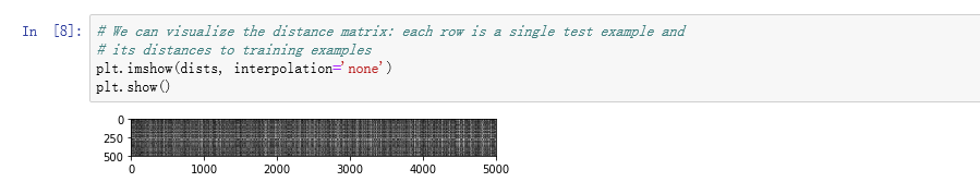
可视化距离矩阵

KNN不需要训练，直接进行预测，k=1

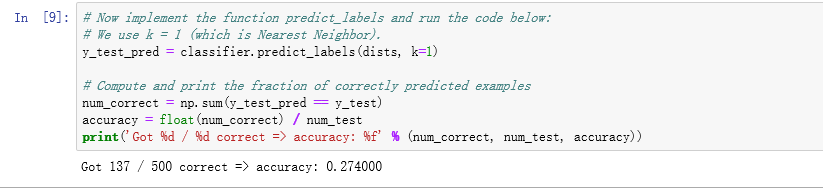
准确率为：0.274，低。

令k=5预测

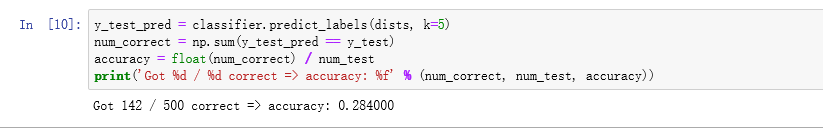
准确率为：0.284,较k=1时稍高。

在一个loop中完成L2距离计算，并用F范数与两个loop时的结果比较验证正确性

不使用loop计算L2距离

之后比较三种方法的速度，很明显不使用loop速度最快

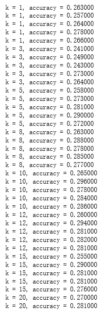
交叉验证：
将训练集分成5等分，观察不同k值下的分类精度

打印出来的结果


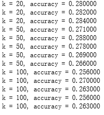
将所得结果画出精度图

从图中可以看出，最高精度在k=10，29%左右
所以令最佳k=10

所得的最佳精度为142/500，28.4%左右，精度较低。

PART two——Multiclass Support Vector Machine

import random
import numpy as np
from cs231n.data_utils import load_CIFAR10
import matplotlib.pyplot as plt

from __future__ import print_function

#基本设定 让matplotlib画的图出现在notebook页面上，而不是新建一个画图窗口．
%matplotlib inline
plt.rcParams['figure.figsize'] = (10.0, 8.0) # 设置默认的绘图窗口大小
plt.rcParams['image.interpolation'] = 'nearest'
plt.rcParams['image.cmap'] = 'gray'
# 另一个设定 可以使notebook自动重载外部python 模块．[点击此处查看详情][4]
# 也就是说，当从外部文件引入的函数被修改之后，在notebook中调用这个函数，得到的被改过的函数．
%load_ext autoreload
%autoreload 2

加载CIFAR10

# 这里加载数据的代码在 data_utils.py 中，会将data_batch_1到5的数据作为训练集，test_batch作为测试集
cifar10_dir = 'cs231n/datasets/cifar-10-batches-py'
X_train, y_train, X_test, y_test = load_CIFAR10(cifar10_dir)

# 为了对数据有一个认识，打印出训练集和测试集的大小 
print('Training data shape: ', X_train.shape)
print('Training labels shape: ', y_train.shape)
print('Test data shape: ', X_test.shape)
print('Test labels shape: ', y_test.shape)

输出结果：

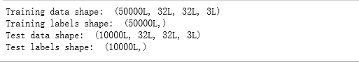
同KNN部分
随机打印每类的图片

# Visualize some examples from the dataset.
# We show a few examples of training images from each class.
classes = ['plane', 'car', 'bird', 'cat', 'deer', 'dog', 'frog', 'horse', 'ship', 'truck']
num_classes = len(classes)
samples_per_class = 7
for y, cls in enumerate(classes):
    idxs = np.flatnonzero(y_train == y)
    idxs = np.random.choice(idxs, samples_per_class, replace=False)
    for i, idx in enumerate(idxs):
        plt_idx = i * num_classes + y + 1
        plt.subplot(samples_per_class, num_classes, plt_idx)
        plt.imshow(X_train[idx].astype('uint8'))
        plt.axis('off')
        if i == 0:
            plt.title(cls)
plt.show()

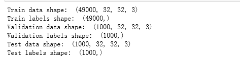
之后将数据集分割成训练集、验证集和测试集

num_training = 49000
num_validation = 1000
num_test = 1000
num_dev = 500

# 验证集将会是从原始的训练集中分割出来的长度为 num_validation 的数据样本点
mask = range(num_training, num_training + num_validation)
X_val = X_train[mask]
y_val = y_train[mask]

# 训练集是原始的训练集中前 num_train 个样本
mask = range(num_training)
X_train = X_train[mask]
y_train = y_train[mask]

# 我们也可以从训练集中随机抽取一小部分的数据点作为开发集
mask = np.random.choice(num_training, num_dev, replace=False)
X_dev = X_train[mask]
y_dev = y_train[mask]

# 使用前 num_test 个测试集点作为测试集
mask = range(num_test)
X_test = X_test[mask]
y_test = y_test[mask]

print('Train data shape: ', X_train.shape)
print('Train labels shape: ', y_train.shape)
print('Validation data shape: ', X_val.shape)
print('Validation labels shape: ', y_val.shape)
print('Test data shape: ', X_test.shape)
print('Test labels shape: ', y_test.shape)

结果为;

将原始数据转化成二维数据

#np.reshape(input_array, (k,-1)), 其中k为除了最后一维的维数，-1表示并不人为指定，由k和原始数据的大小来确定最后一维的长度．
#将所有样本，各自拉成一个行向量，所构成的二维矩阵，每一行就是一个样本，即一行有32X32X3个数，每个数表示一个特征。
X_train = np.reshape(X_train, (X_train.shape[0], -1))
X_val = np.reshape(X_val, (X_val.shape[0], -1))
X_test = np.reshape(X_test, (X_test.shape[0], -1))
X_dev = np.reshape(X_dev, (X_dev.shape[0], -1))
print('Training data shape: ', X_train.shape)
print('Validation data shape: ', X_val.shape)
print('Test data shape: ', X_test.shape)
print('dev data shape: ', X_dev.shape)

输出：

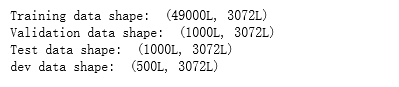
由原来的32323变成了1*3072.

预处理，减去图像平均值：

# 首先，基于训练数据，计算图像的平均值
mean_image = np.mean(X_train, axis=0)#计算每一列特征的平均值，共32x32x3个特征
print(mean_image.shape)
print(mean_image[:10]) # 查看一下特征的数据
plt.figure(figsize=(4,4))#指定画图的框图大小
plt.imshow(mean_image.reshape((32,32,3)).astype('uint8')) # 将平均值可视化出来。
plt.show()

输出结果

# 然后: 训练集和测试集图像分别减去均值#
X_train -= mean_image
X_val -= mean_image
X_test -= mean_image
X_dev -= mean_image
# 最后，在X中添加一列1作为偏置维度，这样我们在优化时候只要考虑一个权重矩阵W就可以啦．
X_train = np.hstack([X_train, np.ones((X_train.shape[0], 1))])
X_val = np.hstack([X_val, np.ones((X_val.shape[0], 1))])
X_test = np.hstack([X_test, np.ones((X_test.shape[0], 1))])
X_dev = np.hstack([X_dev, np.ones((X_dev.shape[0], 1))])
print(X_train.shape, X_val.shape, X_test.shape, X_dev.shape)

输出

SVM 分类器

from cs231n.classifiers.linear_svm import svm_loss_naive
import time

# 生成一个很小的SVM随机权重矩阵
# 真的很小，先标准正态随机然后乘0.0001
W = np.random.randn(3073, 10) * 0.0001 

loss, grad = svm_loss_naive(W, X_dev, y_dev, 0.000005)  # 从dev数据集种的样本抽样计算的loss是。。。大概估计下多少，随机几次，loss在8至9之间
print('loss: %f' % (loss, ))

loss：9.260860

验证梯度结果

# 实现梯度之后，运行下面的代码重新计算梯度．
# 输出是grad_check_sparse函数的结果,2种情况下，可以看出，其实2种算法误差已经几乎不计了。。。
loss, grad = svm_loss_naive(W, X_dev, y_dev, 0.0)
# 对随机选的几个维度计算数值梯度，并把它和你计算的解析梯度比较．所有维度应该几乎相等．
from cs231n.gradient_check import grad_check_sparse
f = lambda w: svm_loss_naive(w, X_dev, y_dev, 0.0)[0]
grad_numerical = grad_check_sparse(f, W, grad)
# 再次验证梯度．这次使用正则项．你肯定没有忘记正则化梯度吧~
print('turn on reg')
loss, grad = svm_loss_naive(W, X_dev, y_dev, 5e1)
f = lambda w: svm_loss_naive(w, X_dev, y_dev, 5e1)[0]
grad_numerical = grad_check_sparse(f, W, grad)

输出：

numerical: -26.580693 analytic: -26.571774, relative error: 1.677865e-04
numerical: 7.909919 analytic: 7.909919, relative error: 6.185816e-12
numerical: 16.401381 analytic: 16.401381, relative error: 7.886468e-12
numerical: 12.210101 analytic: 12.155959, relative error: 2.222038e-03
numerical: 31.038671 analytic: 31.038671, relative error: 2.021494e-12
numerical: -33.443957 analytic: -33.443957, relative error: 1.354535e-11
numerical: 12.178116 analytic: 12.155992, relative error: 9.091910e-04
numerical: 10.061250 analytic: 10.061250, relative error: 1.062980e-11
numerical: -8.362917 analytic: -8.362917, relative error: 9.862139e-12
numerical: 59.056812 analytic: 59.056812, relative error: 4.051852e-12
numerical: 13.010947 analytic: 13.010947, relative error: 2.710146e-12
numerical: 6.731814 analytic: 6.688705, relative error: 3.212125e-03
numerical: -8.759590 analytic: -8.815313, relative error: 3.170616e-03
numerical: 17.957518 analytic: 17.957518, relative error: 2.976116e-11
numerical: 11.112869 analytic: 11.112869, relative error: 2.990886e-11
numerical: 11.234050 analytic: 11.234050, relative error: 2.029875e-11
numerical: -15.436333 analytic: -15.439644, relative error: 1.072401e-04
numerical: -27.464723 analytic: -27.498514, relative error: 6.147939e-04
numerical: -5.350127 analytic: -5.350127, relative error: 3.698055e-11
numerical: 19.201635 analytic: 19.266104, relative error: 1.675918e-03

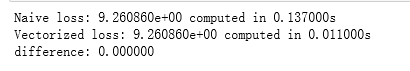
完成 svm_loss_vectorized 方法

# Next implement the function svm_loss_vectorized; for now only compute the loss;
# we will implement the gradient in a moment.
tic = time.time()
loss_naive, grad_naive = svm_loss_naive(W, X_dev, y_dev, 0.000005)
toc = time.time()
print('Naive loss: %e computed in %fs' % (loss_naive, toc - tic))

from cs231n.classifiers.linear_svm import svm_loss_vectorized
tic = time.time()
loss_vectorized, _ = svm_loss_vectorized(W, X_dev, y_dev, 0.000005)
toc = time.time()
print('Vectorized loss: %e computed in %fs' % (loss_vectorized, toc - tic))

# The losses should match but your vectorized implementation should be much faster.
print('difference: %f' % (loss_naive - loss_vectorized))

输出

# 使用向量来计算损失函数的梯度．
# 朴素方法和向量法的结果应该是一样的，但是向量法会更快一点．

tic = time.time()
_, grad_naive = svm_loss_naive(W, X_dev, y_dev, 0.000005)
toc = time.time()
print('Naive loss and gradient: computed in %fs' % (toc - tic))

tic = time.time()
_, grad_vectorized = svm_loss_vectorized(W, X_dev, y_dev, 0.000005)
toc = time.time()
print('Vectorized loss and gradient: computed in %fs' % (toc - tic))

# The loss is a single number, so it is easy to compare the values computed
# by the two implementations. The gradient on the other hand is a matrix, so
# we use the Frobenius norm to compare them.
difference = np.linalg.norm(grad_naive - grad_vectorized, ord='fro')
print('difference: %f' % difference)

输出：可以看出，向量法比朴素方法稍快

随机梯度下降

# In the file linear_classifier.py, implement SGD in the function
# LinearClassifier.train() and then run it with the code below.
from cs231n.classifiers import LinearSVM
svm = LinearSVM()
tic = time.time()
loss_hist = svm.train(X_train, y_train, learning_rate=1e-7, reg=2.5e4,
                      num_iters=1500, verbose=True)
toc = time.time()
print('That took %fs' % (toc - tic))

iteration 0 / 1500: loss 791.476480
iteration 100 / 1500: loss 288.685023
iteration 200 / 1500: loss 108.462208
iteration 300 / 1500: loss 42.626097
iteration 400 / 1500: loss 18.990406
iteration 500 / 1500: loss 10.066142
iteration 600 / 1500: loss 7.207224
iteration 700 / 1500: loss 6.043331
iteration 800 / 1500: loss 5.527581
iteration 900 / 1500: loss 5.037615
iteration 1000 / 1500: loss 4.932641
iteration 1100 / 1500: loss 5.412060
iteration 1200 / 1500: loss 5.390348
iteration 1300 / 1500: loss 5.518095
iteration 1400 / 1500: loss 5.047453
That took 9.718000s

# A useful debugging strategy is to plot the loss as a function of
# iteration number:
plt.plot(loss_hist)
plt.xlabel('Iteration number')
plt.ylabel('Loss value')
plt.show()

# Write the LinearSVM.predict function and evaluate the performance on both the
# training and validation set
y_train_pred = svm.predict(X_train)
print('training accuracy: %f' % (np.mean(y_train == y_train_pred), ))
y_val_pred = svm.predict(X_val)
print('validation accuracy: %f' % (np.mean(y_val == y_val_pred), ))

输出：

training accuracy: 0.362224
validation accuracy: 0.372000

使用验证集去调整超参数（正则化强度和学习率）

# Use the validation set to tune hyperparameters (regularization strength and
# learning rate). You should experiment with different ranges for the learning
# rates and regularization strengths; if you are careful you should be able to
# get a classification accuracy of about 0.4 on the validation set.
learning_rates = [1.7e-7] # The lr 5e-5 makes GD overflow at W*W
regularization_strengths = [1.2e4]

# results is dictionary mapping tuples of the form
# (learning_rate, regularization_strength) to tuples of the form
# (training_accuracy, validation_accuracy). The accuracy is simply the fraction
# of data points that are correctly classified.
results = {}
best_val = -1   # The highest validation accuracy that we have seen so far.
best_svm = None # The LinearSVM object that achieved the highest validation rate.

################################################################################
# TODO:                                                                        #
# Write code that chooses the best hyperparameters by tuning on the validation #
# set. For each combination of hyperparameters, train a linear SVM on the      #
# training set, compute its accuracy on the training and validation sets, and  #
# store these numbers in the results dictionary. In addition, store the best   #
# validation accuracy in best_val and the LinearSVM object that achieves this  #
# accuracy in best_svm.                                                        #
#                                                                              #
# Hint: You should use a small value for num_iters as you develop your         #
# validation code so that the SVMs don't take much time to train; once you are #
# confident that your validation code works, you should rerun the validation   #
# code with a larger value for num_iters.                                      #
################################################################################
from cs231n.classifiers import LinearSVM

for lr in learning_rates:
    for reg in regularization_strengths:
        svm = LinearSVM()
        svm.train(X_train, y_train, learning_rate=lr, reg=reg, num_iters=1000, verbose=False)
        y_train_pred = svm.predict(X_train)
        train_accuracy = np.mean(y_train == y_train_pred)
        y_val_pred = svm.predict(X_val)
        val_accuracy = np.mean(y_val == y_val_pred)
        results[(lr, reg)] = (train_accuracy, val_accuracy)
        if best_val < val_accuracy:
            best_val = val_accuracy
            best_svm = svm
################################################################################
#                              END OF YOUR CODE                                #
################################################################################
    
# Print out results.
for lr, reg in sorted(results):
    train_accuracy, val_accuracy = results[(lr, reg)]
    print('lr %e reg %e train accuracy: %f val accuracy: %f' % (
                lr, reg, train_accuracy, val_accuracy))
    
print('best validation accuracy achieved during cross-validation: %f' % best_val)

lr 7.500000e-08 reg 3.000000e+04 train accuracy: 0.368918 val accuracy: 0.370000
lr 7.500000e-08 reg 3.250000e+04 train accuracy: 0.364408 val accuracy: 0.385000
lr 7.500000e-08 reg 3.500000e+04 train accuracy: 0.371653 val accuracy: 0.380000
lr 7.500000e-08 reg 3.750000e+04 train accuracy: 0.365429 val accuracy: 0.371000
lr 7.500000e-08 reg 4.000000e+04 train accuracy: 0.359918 val accuracy: 0.372000
lr 7.500000e-08 reg 4.250000e+04 train accuracy: 0.367714 val accuracy: 0.380000
lr 7.500000e-08 reg 4.500000e+04 train accuracy: 0.365265 val accuracy: 0.378000
lr 7.500000e-08 reg 4.750000e+04 train accuracy: 0.358878 val accuracy: 0.368000
lr 7.500000e-08 reg 5.000000e+04 train accuracy: 0.357939 val accuracy: 0.373000
lr 1.250000e-07 reg 3.000000e+04 train accuracy: 0.363469 val accuracy: 0.376000
lr 1.250000e-07 reg 3.250000e+04 train accuracy: 0.357796 val accuracy: 0.369000
lr 1.250000e-07 reg 3.500000e+04 train accuracy: 0.357449 val accuracy: 0.364000
lr 1.250000e-07 reg 3.750000e+04 train accuracy: 0.366327 val accuracy: 0.370000
lr 1.250000e-07 reg 4.000000e+04 train accuracy: 0.361000 val accuracy: 0.365000
lr 1.250000e-07 reg 4.250000e+04 train accuracy: 0.363143 val accuracy: 0.368000
lr 1.250000e-07 reg 4.500000e+04 train accuracy: 0.352551 val accuracy: 0.369000
lr 1.250000e-07 reg 4.750000e+04 train accuracy: 0.343816 val accuracy: 0.364000
lr 1.250000e-07 reg 5.000000e+04 train accuracy: 0.359531 val accuracy: 0.375000
lr 1.500000e-07 reg 3.000000e+04 train accuracy: 0.365878 val accuracy: 0.381000
lr 1.500000e-07 reg 3.250000e+04 train accuracy: 0.358347 val accuracy: 0.377000
lr 1.500000e-07 reg 3.500000e+04 train accuracy: 0.363082 val accuracy: 0.376000
lr 1.500000e-07 reg 3.750000e+04 train accuracy: 0.361204 val accuracy: 0.364000
lr 1.500000e-07 reg 4.000000e+04 train accuracy: 0.361286 val accuracy: 0.360000
lr 1.500000e-07 reg 4.250000e+04 train accuracy: 0.352184 val accuracy: 0.355000
lr 1.500000e-07 reg 4.500000e+04 train accuracy: 0.352551 val accuracy: 0.360000
lr 1.500000e-07 reg 4.750000e+04 train accuracy: 0.356224 val accuracy: 0.364000
lr 1.500000e-07 reg 5.000000e+04 train accuracy: 0.353918 val accuracy: 0.368000
lr 2.000000e-07 reg 3.000000e+04 train accuracy: 0.360245 val accuracy: 0.375000
lr 2.000000e-07 reg 3.250000e+04 train accuracy: 0.363857 val accuracy: 0.372000
lr 2.000000e-07 reg 3.500000e+04 train accuracy: 0.365939 val accuracy: 0.390000
lr 2.000000e-07 reg 3.750000e+04 train accuracy: 0.343143 val accuracy: 0.349000
lr 2.000000e-07 reg 4.000000e+04 train accuracy: 0.354551 val accuracy: 0.367000
lr 2.000000e-07 reg 4.250000e+04 train accuracy: 0.348531 val accuracy: 0.358000
lr 2.000000e-07 reg 4.500000e+04 train accuracy: 0.352429 val accuracy: 0.361000
lr 2.000000e-07 reg 4.750000e+04 train accuracy: 0.347796 val accuracy: 0.348000
lr 2.000000e-07 reg 5.000000e+04 train accuracy: 0.343694 val accuracy: 0.360000
best validation accuracy achieved during cross-validation: 0.390000

Visualize the cross-validation results

import math
x_scatter = [math.log10(x[0]) for x in results]
y_scatter = [math.log10(x[1]) for x in results]

#画出训练准确率
marker_size = 100
colors = [results[x][0] for x in results]
plt.subplot(2, 1, 1)
plt.scatter(x_scatter, y_scatter, marker_size, c=colors)
plt.colorbar()
plt.xlabel('log learning rate')
plt.ylabel('log regularization strength')
plt.title('CIFAR-10 training accuracy')

#画出验证准确率
colors = [results[x][1] for x in results] # default size of markers is 20
plt.subplot(2, 1, 2)
plt.scatter(x_scatter, y_scatter, marker_size, c=colors)
plt.colorbar()
plt.xlabel('log learning rate')
plt.ylabel('log regularization strength')
plt.title('CIFAR-10 validation accuracy')
plt.tight_layout() # 调整子图间距
plt.show()

结果如图：

在测试集上评价最好的svm的表现

# Evaluate the best svm on test set
y_test_pred = best_svm.predict(X_test)
test_accuracy = np.mean(y_test == y_test_pred)
print('linear SVM on raw pixels final test set accuracy: %f' % test_accuracy)

输出结果：
linear SVM on raw pixels final test set accuracy: 0.360000

#对于每一类，可视化学习到的权重
#依赖于你对学习权重和正则化强度的选择，这些可视化效果或者很明显或者不明显。
w = best_svm.W[:-1,:] # strip out the bias
w = w.reshape(32, 32, 3, 10)
w_min, w_max = np.min(w), np.max(w)
classes = ['plane', 'car', 'bird', 'cat', 'deer', 'dog', 'frog', 'horse', 'ship', 'truck']
for i in range(10):
    plt.subplot(2, 5, i + 1)

    # Rescale the weights to be between 0 and 255
    wimg = 255.0 * (w[:, :, :, i].squeeze() - w_min) / (w_max - w_min)
    plt.imshow(wimg.astype('uint8'))
    plt.axis('off')
    plt.title(classes[i])

可视化结果