线性回归分析(python3)
1、python固定导入的包
# 工具:python3

#固定导入
import numpy as np               #科学计算基础库,多维数组对象ndarray
import pandas as pd              #数据处理库,DataFrame(二维数组)
import matplotlib as mpl         #画图基础库
import matplotlib.pyplot as plt  #最常用的绘图库
from scipy import stats          #scipy库的stats模块

mpl.rcParams["font.family"]="SimHei"  #使用支持的黑体中文字体
mpl.rcParams["axes.unicode_minus"]=False # 用来正常显示负号  "-"
plt.rcParams['font.sans-serif']=['SimHei'] # 用来正常显示中文标签
# % matplotlib inline  #jupyter中用于直接嵌入图表,不用plt.show()
import warnings
warnings.filterwarnings("ignore") #用于排除警告

#用于显示使用库的版本
print("numpy_" + np.__version__)
print("pandas_" + pd.__version__)
print("matplotlib_"+ mpl.__version__)
numpy_1.17.4
pandas_0.23.4
matplotlib_2.2.3
2、常见的回归函数


3、线性回归
Y= aX + b + e ,e表示残差
线性回归:分析结论的前提:数据满足统计假设
- 正态性:预测变量固定时,因变量正态分布
- 独立性:因变量互相独立
- 线性:因变量与自变量线性(残差白噪声)
- 同方差性:残差方差均匀
(1)、scipy.optimize.curve_fit():回归函数拟合
from scipy.optimize import curve_fit   #回归函数拟合包

def func(x,a,b):
    y = a*x + b
    return y
x= np.array([150,200,250,350,300,400,600])
ydata=np.array([6450,7450,8450,9450,11450,15450,18450])
popt,pcov=curve_fit(func,x,ydata)
print(curve_fit(func,x,ydata)) #拟合函数 y = 28.03191489*x + 2011.17021277

plt.title('分布图')
plt.xlabel('x')
plt.ylabel('y')
plt.plot(x,ydata,'bo',x,func(x,popt[0],popt[1]),'r-')
plt.legend(["ydata","y拟合"],loc="best", frameon=False, ncol=1)
plt.show()
(array([  28.03191489, 2011.17021277]), array([[ 1.81614985e+01, -5.83762446e+03],
       [-5.83762446e+03,  2.22478353e+06]]))

(2)、scipy.stats.linregress(): 线性拟合
from scipy import stats  #线性回归包
x= np.array([150,200,250,350,300,400,600])
ydata=np.array([6450,7450,8450,9450,11450,15450,18450])
slope, intercept, r_value, p_value, std_err = stats.linregress(x,ydata)
#a   ,  b         r ,    p ,      标准误
print(stats.linregress(x,ydata))
y = slope*x + intercept #拟合函数
LinregressResult(slope=28.03191489361702, intercept=2011.1702127659555,
rvalue=0.9467887456768281, pvalue=0.0012189021752212815, stderr=4.261630957224319)
(3)、statsmodels.formula.api.OLS():普通最小二乘模型拟合- - 常用
tips = pd.read_csv(r"E:\tips.txt",sep='\t',encoding='utf-8') #导入txt格式数据
display(tips.sample(3)) #随机抽取3行数据
import statsmodels.formula.api as sm  #statsmodels.formula.api.ols 回归模型库
model = sm.OLS(tips["total_bill"], tips["tip"]) # OLS 是普通最小二乘,sm 中还有很多其它方法解决不同的问题
# total_bill:因变量, tip:自变量
result = model.fit()    # 做拟合

print(result.summary()) #返回拟合总结信息

print(result.params)  # 对应的各个变量的权重

resid = result.resid  # 输出残差
print(type(resid))    # <class 'pandas.core.series.Series'>
print(stats.normaltest(result.resid.values)) #对残差进行正态分布检验,p<阀值,拒绝原假设,则是正态分布

figure = plt.figure(num="画布1",figsize=(8,4),dpi=80,facecolor="gray",edgecolor="blue",frameon=True)
axes1=figure.add_subplot(2,2,1)
plt.title("残差图")
axes1.plot(result.resid) #看看残差图

axes2=figure.add_subplot(2,2,2)
plt.title('分布/拟合图')
plt.xlabel('tip')
plt.ylabel('total_bill')
axes2.plot(tips["tip"],tips["total_bill"],'bo',tips["tip"],result.params[0]*tips["tip"],'r-')
plt.legend(["total_bill","total_bill拟合"],loc="best", frameon=False, ncol=2)
plt.show()

# '''
# 模型解释:
# result.summary()的输出解释:R-squared:0.892,Adj. R-squared:0.891 都比较大,说明模型是比较显著的,
# tip的权值检验p:0.000,非常小,拒绝原假设,说明系数的正确性也是非常显著的。
# stats.normaltest(result.resid.values) :对残差进行正态分布检验,p<阀值,说明残差也是符合要求。
# 模型可用。
# 模型公式:total_bill = 6.2052 * tip
# '''
| total_bill | tip | sex | smoker | day | time | size | |
|---|---|---|---|---|---|---|---|
| 92 | 5.75 | 1.00 | Female | Yes | Fri | Dinner | 2 |
| 139 | 13.16 | 2.75 | Female | No | Thur | Lunch | 2 |
| 136 | 10.33 | 2.00 | Female | No | Thur | Lunch | 2 |
                            OLS Regression Results
==============================================================================
Dep. Variable:             total_bill   R-squared:                       0.892
Model:                            OLS   Adj. R-squared:                  0.891
Method:                 Least Squares   F-statistic:                     2004.
Date:                Sun, 16 Feb 2020   Prob (F-statistic):          2.26e-119
Time:                        18:07:20   Log-Likelihood:                -825.57
No. Observations:                 244   AIC:                             1653.
Df Residuals:                     243   BIC:                             1657.
Df Model:                           1
Covariance Type:            nonrobust
==============================================================================
                 coef    std err          t      P>|t|      [0.025      0.975]
------------------------------------------------------------------------------
tip            6.2052      0.139     44.771      0.000       5.932       6.478
==============================================================================
Omnibus:                       33.937   Durbin-Watson:                   2.112
Prob(Omnibus):                  0.000   Jarque-Bera (JB):               71.569
Skew:                           0.688   Prob(JB):                     2.88e-16
Kurtosis:                       5.269   Cond. No.                         1.00
==============================================================================

Warnings:
[1] Standard Errors assume that the covariance matrix of the errors is correctly specified.
tip    6.205158
dtype: float64
<class 'pandas.core.series.Series'>
NormaltestResult(statistic=33.937192138902724, pvalue=4.2720109911999064e-08)
![[外链图片转存失败,源站可能有防盗链机制,建议将图片保存下来直接上传(img-BVh9drVQ-1581847738893)(output_12_2.png)]](https://img-blog.csdnimg.cn/2020021618134319.png)
statsmodels.formula.api.ols():还可以采取公式的方式。
np.random.seed(123456789)
N = 100
x1 = np.random.randn(N) # 自变量
x2 = np.random.randn(N)
data = pd.DataFrame({"x1": x1, "x2": x2})
def y_true(x1, x2):
    return 1  + 2 * x1 + 3 * x2 + 4 * x1 * x2
data["y_true"] = y_true(x1, x2) # 因变量
e = np.random.randn(N) # 标准正态分布
data["y"] = data["y_true"] + e # 加些噪音,加些扰动,噪音是符合标准正态分布的
data.head(3)

import statsmodels.formula.api as sm  #statsmodels.formula.api.ols 回归模型库
model = sm.ols("y ~x1 + x2", data) # 这里没有写截距,截距是默认存在的
# model = sm.ols("y ~ -1 + x1 + x2", data) # 这里加上-1,表示不加截距
result = model.fit()
print(result.summary())
                            OLS Regression Results
==============================================================================
Dep. Variable:                      y   R-squared:                       0.380
Model:                            OLS   Adj. R-squared:                  0.367
Method:                 Least Squares   F-statistic:                     29.76
Date:                Sun, 16 Feb 2020   Prob (F-statistic):           8.36e-11
Time:                        18:07:20   Log-Likelihood:                -271.52
No. Observations:                 100   AIC:                             549.0
Df Residuals:                      97   BIC:                             556.9
Df Model:                           2
Covariance Type:            nonrobust
==============================================================================
                 coef    std err          t      P>|t|      [0.025      0.975]
------------------------------------------------------------------------------
Intercept      0.9868      0.382      2.581      0.011       0.228       1.746
x1             1.0810      0.391      2.766      0.007       0.305       1.857
x2             3.0793      0.432      7.134      0.000       2.223       3.936
==============================================================================
Omnibus:                       19.951   Durbin-Watson:                   1.682
Prob(Omnibus):                  0.000   Jarque-Bera (JB):               49.964
Skew:                          -0.660   Prob(JB):                     1.41e-11
Kurtosis:                       6.201   Cond. No.                         1.32
==============================================================================

Warnings:
[1] Standard Errors assume that the covariance matrix of the errors is correctly specified.
4、回归诊断流程
![[外链图片转存失败,源站可能有防盗链机制,建议将图片保存下来直接上传(img-Oq6DgmrB-1581847738894)(attachment:image.png)]](https://img-blog.csdnimg.cn/20200216181423505.png?x-oss-process=image/watermark,type_ZmFuZ3poZW5naGVpdGk,shadow_10,text_aHR0cHM6Ly9ibG9nLmNzZG4ubmV0L3dlaXhpbl80MTY4NTM4OA==,size_16,color_FFFFFF,t_70)
对于多变量的时候,非常复杂,我们往往会去尝试很多模型,然后选择最优模型,常用剔除法(倒退法)
data = pd.read_csv(r"E:\regdata1.csv",sep=',',encoding='utf-8') #导入csv格式数据
display(tips.sample(3)) #随机抽取3行数据
import statsmodels.formula.api as sm  #statsmodels.formula.api.ols 回归模型库
result=sm.ols(formula="y1~x1+x2+x3+x5+x6",data=data).fit()
print(result.summary()) #返回拟合总结信息
# x2 的 p:0.291 ,先去除看看
| total_bill | tip | sex | smoker | day | time | size | |
|---|---|---|---|---|---|---|---|
| 20 | 17.92 | 4.08 | Male | No | Sat | Dinner | 2 |
| 99 | 12.46 | 1.50 | Male | No | Fri | Dinner | 2 |
| 29 | 19.65 | 3.00 | Female | No | Sat | Dinner | 2 |
                            OLS Regression Results
==============================================================================
Dep. Variable:                     y1   R-squared:                       0.894
Model:                            OLS   Adj. R-squared:                  0.876
Method:                 Least Squares   F-statistic:                     50.44
Date:                Sun, 16 Feb 2020   Prob (F-statistic):           1.05e-13
Time:                        18:07:21   Log-Likelihood:                -108.08
No. Observations:                  36   AIC:                             228.2
Df Residuals:                      30   BIC:                             237.7
Df Model:                           5
Covariance Type:            nonrobust
==============================================================================
                 coef    std err          t      P>|t|      [0.025      0.975]
------------------------------------------------------------------------------
Intercept      0.6359      5.862      0.108      0.914     -11.336      12.608
x1             1.4037      0.249      5.642      0.000       0.896       1.912
x2            -0.0676      0.063     -1.074      0.291      -0.196       0.061
x3            -0.2036      0.160     -1.271      0.214      -0.531       0.124
x5            -0.6946      0.255     -2.722      0.011      -1.216      -0.173
x6             4.6154      0.339     13.612      0.000       3.923       5.308
==============================================================================
Omnibus:                       14.780   Durbin-Watson:                   2.071
Prob(Omnibus):                  0.001   Jarque-Bera (JB):               16.290
Skew:                           1.306   Prob(JB):                     0.000290
Kurtosis:                       5.009   Cond. No.                         175.
==============================================================================

Warnings:
[1] Standard Errors assume that the covariance matrix of the errors is correctly specified.
result=sm.ols(formula="y1~x1+x3+x5+x6",data=data).fit()
print(result.summary()) #返回拟合总结信息
# x3 的 p:0.222,去除看看
                            OLS Regression Results
==============================================================================
Dep. Variable:                     y1   R-squared:                       0.890
Model:                            OLS   Adj. R-squared:                  0.875
Method:                 Least Squares   F-statistic:                     62.45
Date:                Sun, 16 Feb 2020   Prob (F-statistic):           2.17e-14
Time:                        18:07:21   Log-Likelihood:                -108.76
No. Observations:                  36   AIC:                             227.5
Df Residuals:                      31   BIC:                             235.4
Df Model:                           4
Covariance Type:            nonrobust
==============================================================================
                 coef    std err          t      P>|t|      [0.025      0.975]
------------------------------------------------------------------------------
Intercept     -0.5756      5.767     -0.100      0.921     -12.337      11.186
x1             1.4259      0.249      5.737      0.000       0.919       1.933
x3            -0.2004      0.161     -1.248      0.222      -0.528       0.127
x5            -0.6967      0.256     -2.723      0.011      -1.218      -0.175
x6             4.6147      0.340     13.577      0.000       3.921       5.308
==============================================================================
Omnibus:                       12.513   Durbin-Watson:                   2.147
Prob(Omnibus):                  0.002   Jarque-Bera (JB):               12.554
Skew:                           1.179   Prob(JB):                      0.00188
Kurtosis:                       4.675   Cond. No.                         137.
==============================================================================

Warnings:
[1] Standard Errors assume that the covariance matrix of the errors is correctly specified.
result=sm.ols(formula="y1~x1+x5+x6",data=data).fit()
print(result.summary()) #返回拟合总结信息
# Intercept 的 p:0.990,去除看看
                            OLS Regression Results
==============================================================================
Dep. Variable:                     y1   R-squared:                       0.884
Model:                            OLS   Adj. R-squared:                  0.873
Method:                 Least Squares   F-statistic:                     81.34
Date:                Sun, 16 Feb 2020   Prob (F-statistic):           4.65e-15
Time:                        18:07:21   Log-Likelihood:                -109.64
No. Observations:                  36   AIC:                             227.3
Df Residuals:                      32   BIC:                             233.6
Df Model:                           3
Covariance Type:            nonrobust
==============================================================================
                 coef    std err          t      P>|t|      [0.025      0.975]
------------------------------------------------------------------------------
Intercept     -0.0701      5.802     -0.012      0.990     -11.889      11.749
x1             1.4427      0.250      5.763      0.000       0.933       1.953
x5            -0.8027      0.243     -3.298      0.002      -1.298      -0.307
x6             4.5462      0.338     13.437      0.000       3.857       5.235
==============================================================================
Omnibus:                       16.154   Durbin-Watson:                   2.089
Prob(Omnibus):                  0.000   Jarque-Bera (JB):               19.372
Skew:                           1.343   Prob(JB):                     6.21e-05
Kurtosis:                       5.389   Cond. No.                         131.
==============================================================================

Warnings:
[1] Standard Errors assume that the covariance matrix of the errors is correctly specified.
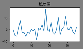
result=sm.ols(formula="y1~-1+x1+x5+x6",data=data).fit() #加-1表示不要截距
print(result.summary()) #返回拟合总结信息

print(result.params)  # 对应的各个变量的权重

resid = result.resid  # 输出残差
print(type(resid))    # <class 'pandas.core.series.Series'>
print(stats.normaltest(result.resid.values)) #对残差进行正态分布检验,p<阀值,拒绝原假设,则是正态分布

figure = plt.figure(num="画布1",figsize=(8,4),dpi=80,facecolor="gray",edgecolor="blue",frameon=True)
axes1=figure.add_subplot(2,2,1)
plt.title("残差图")
axes1.plot(result.resid) #看看残差图
plt.show()
                            OLS Regression Results
==============================================================================
Dep. Variable:                     y1   R-squared:                       0.995
Model:                            OLS   Adj. R-squared:                  0.994
Method:                 Least Squares   F-statistic:                     2064.
Date:                Sun, 16 Feb 2020   Prob (F-statistic):           1.33e-37
Time:                        18:07:21   Log-Likelihood:                -109.64
No. Observations:                  36   AIC:                             225.3
Df Residuals:                      33   BIC:                             230.0
Df Model:                           3
Covariance Type:            nonrobust
==============================================================================
                 coef    std err          t      P>|t|      [0.025      0.975]
------------------------------------------------------------------------------
x1             1.4411      0.211      6.845      0.000       1.013       1.869
x5            -0.8040      0.215     -3.737      0.001      -1.242      -0.366
x6             4.5432      0.233     19.539      0.000       4.070       5.016
==============================================================================
Omnibus:                       16.185   Durbin-Watson:                   2.089
Prob(Omnibus):                  0.000   Jarque-Bera (JB):               19.437
Skew:                           1.344   Prob(JB):                     6.02e-05
Kurtosis:                       5.394   Cond. No.                         6.78
==============================================================================

Warnings:
[1] Standard Errors assume that the covariance matrix of the errors is correctly specified.
x1    1.441105
x5   -0.803997
x6    4.543234
dtype: float64
<class 'pandas.core.series.Series'>
NormaltestResult(statistic=16.185229150896554, pvalue=0.0003057892020932761)
5、避免过度拟合:
- 原则简单模型和复杂模型都通过检验时选择简单模型
- R^2增大的同时,调整后的R^2_p也应该同样增大

