这是一次统计学的作业
线性模型
今天我们所知道的回归是由达尔文(Charles Darwin)的表兄弟Francis Galton发明的。Galton
于1877年完成了第一次回归预测,目的是根据上一代豌豆种子(双亲)的尺寸来预测下一代豌
豆种子(孩子)的尺寸。Galton在大量对象上应用了回归分析,甚至包括人的身高。他注意到,
如果双亲的高度比平均高度高,他们的子女也倾向于比平均高度高,但尚不及双亲。孩子的高
度向着平均高度回退(回归)。Galton在多项研究上都注意到这个现象,所以尽管这个英文单
词跟数值预测没有任何关系,但这种研究方法仍被称作回归.
第一步:准备数据
建立一个函数名字,叫load_data,目的为打开一个TAB键分隔的文本文件,返回值数据与类标。
注意:目标数据集ex0有两三列,第一二列为数据,三列为标签
import numpy as np
#load data from file导入txt数据
def load_data(filename):
    dataset = []
    label = []
    file = open(filename)
    for line in file.readlines():
        lineArr = line.strip().split('\t')
        dataset.append(lineArr[0:2])
        label.append(lineArr[-1])
    return np.array(dataset,dtype=np.float64),\
           np.array(label,dtype=np.float64).reshape(-1,1)
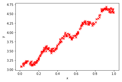
第二步 可视化画图
import matplotlib.pyplot as plt
#导入数据并且可视化一下
x,y = load_data("C:/Users/Nicht_sehen/Desktop/ex0.txt")
print(x.shape,y.shape)
print(x[0],y[0])


plt.scatter(x[:,1],y[:,0],marker='x',color = 'r')
plt.xlabel('x')
plt.ylabel('y')
plt.show()
(200, 2) (200, 1)
[1.       0.067732] [3.176512]
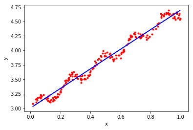
第三步 带入正规方程求解,画画图看拟合效果
#简单的线性回归,使用求导公式就可以求得w的最优值

def normalEquation(X_train,y_train):
    w = np.zeros((X_train.shape[0],1))
    #这里用的伪逆,所以不用判断矩阵的逆存不存在
    w = ((np.linalg.pinv(X_train.T.dot(X_train))).dot(X_train.T)).dot(y_train)
    return w
w = normalEquation(x,y)
print(w)
[[3.00774323]
 [1.69532267]]
#现在可视化一下求得w的效果
plt.scatter(x[:,1],y[:,0],marker='.',color = 'r')
plt.plot(x[:,1],x.dot(w),color = "blue",linestyle = "-")
plt.xlabel('x')
plt.ylabel('y')
plt.show()

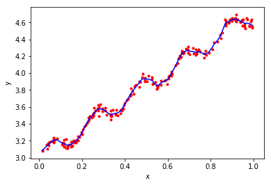
第四步 试试加权最小乘回归
随机生成权重,练习加权最小二乘回归
def gaussi_w(x,y,k=0.1):
    m =np.shape(x)[0]
    w = np.mat(np.eye(m))
    p=np.zeros(m)
    x =np.mat(x)
    for i in range(m):
            for j in range(m):
                s = x[i,]-x[j,]
                w[j,j]=np.exp(s@s.T/(-2.0*k**2))
            xTx = x.T@(w@x)
            xTy = x.T@(w@y)
            wb = np.linalg.pinv(xTx)@xTy
            p[i] = x[i]*wb
    return p


p = gaussi_w(x,y,0.01)
Index = argsort(x[:,1],0)
xsort = x[Index][:]

print(p.shape)
plt.scatter(x[:,1],y[:,0],marker='.',color = 'r')
plt.plot(xsort[:,1],p[Index],color = "blue",linestyle = "-")
plt.xlabel('x')
plt.ylabel('y')
plt.show()
(200,)
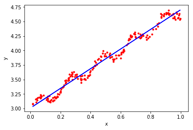
五 岭回归
#当数据的特征非常的多,n>m时,则输入数据X不是满秩矩阵,非满秩矩阵求逆会有问题
#岭回归 == 加入了正则化,缩减权重系数,也就是减少特征值数量

#岭回归公式求解
def ridgeRegress(x,y,lammda = 0.2):
    m,n = x.shape
    I = np.eye((n))
    temp = x.T.dot(x) + lammda * I
    w = np.linalg.pinv(temp).dot(x.T).dot(y)
    return w
w = ridgeRegress(x,y)
print(w)

#现在可视化一下求得w的效果
plt.scatter(x[:,1],y[:,0],marker='.',color = 'r')
plt.plot(x[:,1],x.dot(w),color = "blue",linestyle = "-")
plt.xlabel('x')
plt.ylabel('y')
plt.show()
[[3.00602277]
 [1.69269003]]
再试一种Huber损失、或者Tukey损失函数最小二乘回归
from sklearn.linear_model import HuberRegressor

huber = HuberRegressor().fit(x, y)
p = huber.predict(x)

plt.scatter(x[:,1],y[:,0],marker='.',color = 'r')
plt.plot(x[:,1],p,color = "blue",linestyle = "-")
plt.xlabel('x')
plt.ylabel('y')
plt.show()
六 万能算法ADMM求解Lasso
初学者写时不建议用类
import numpy as np
import matplotlib.pyplot as plt
from math import sqrt, log
## 这个是l1范数截断算子
def Sthresh(x, gamma):
    return np.sign(x)*np.maximum(0, np.absolute(x)-gamma)
def ADMM(A, y):

    m, n = A.shape
    w, v = np.linalg.eig(A.T.dot(A))
    MAX_ITER = 10000
    rho=0.01

    # 求解问题 min 1/2(y - Ax) + l||x||"
    # 初始化
    xhat = np.zeros([n, 1])
    zhat = np.zeros([n, 1])
    u = np.zeros([n, 1])

    # 初始化步长
    l = sqrt(2*log(n, 10))
    AtA = A.T.dot(A)
    Aty = A.T.dot(y)
    # 为了可逆
    Q = AtA + 0.01*np.identity(n)
    Q = np.linalg.inv(Q)

    i = 0

    while(i < MAX_ITER):
        # x 更新
        xhat = Q.dot(Aty + rho*(zhat - u))

        # z 更新 0.1 为可调参数
        zhat = Sthresh(xhat + u, 0.1)

        # 对偶变量更新
        u = u + xhat - zhat

        i = i+1
    return xhat,  l
合成数据试一试
A = np.random.randn(50, 200)

num_non_zeros = 10
positions = np.random.randint(0, 200, num_non_zeros)
amplitudes = 100*np.random.randn(num_non_zeros, 1)
x = np.zeros((200, 1))
x[positions] = amplitudes

y = A.dot(x) + np.random.randn(50, 1)

xhat,  l = ADMM(A, y)

plt.plot(x, label='合成值')
plt.plot(xhat, label = '估计值')

plt.legend(loc = 'upper right')

plt.show()
