数值微分和数值积分一对兄弟给人的第一印象是一件事的两面,但事实上前者是远比后者困难的一件事,数值微分作为一个不适定的问题,在人们认为十分自然的经典做法中却存在着很多坏的特性,接下来我们将看到数值微分无法通过加密网格尺度来提高收敛精度 以及稍有扰动就会对数值微分结果产生非常恶劣的影响 这两个坏消息是如何产生的。
求解函数
f
(
x
)
f(x)
f ( x )
x
0
{{x}_{0}}
x 0
f
′
(
x
0
)
=
lim
h
→
0
f
(
x
0
+
h
)
−
f
(
x
0
)
h
f'({{x}_{0}})=\underset{h\to 0}{\mathop{\lim }}\,\frac{f({{x}_{0}}+h)-f({{x}_{0}})}{h}
f ′ ( x 0 ) = h → 0 lim h f ( x 0 + h ) − f ( x 0 )
设
f
∈
C
2
f\in {{C}^{2}}
f ∈ C 2
f
′
(
x
0
)
≈
f
(
x
0
+
h
)
−
f
(
x
0
)
h
f'({{x}_{0}})\approx \frac{f({{x}_{0}}+h)-f({{x}_{0}})}{h}
f ′ ( x 0 ) ≈ h f ( x 0 + h ) − f ( x 0 )
f
(
x
0
+
h
)
−
f
(
x
0
)
h
−
f
′
(
x
0
)
=
h
2
f
′
′
(
x
0
)
+
O
(
h
2
)
\frac{f({{x}_{0}}+h)-f({{x}_{0}})}{h}-f'({{x}_{0}})=\frac{h}{2}f''({{x}_{0}})+O({{h}^{2}})
h f ( x 0 + h ) − f ( x 0 ) − f ′ ( x 0 ) = 2 h f ′ ′ ( x 0 ) + O ( h 2 )
设
f
∈
C
2
f\in {{C}^{2}}
f ∈ C 2
f
′
(
x
0
)
≈
f
(
x
0
)
−
f
(
x
0
−
h
)
h
f'({{x}_{0}})\approx \frac{f({{x}_{0}})-f({{x}_{0}}-h)}{h}
f ′ ( x 0 ) ≈ h f ( x 0 ) − f ( x 0 − h )
f
(
x
0
)
−
f
(
x
0
−
h
)
h
−
f
′
(
x
0
)
=
−
h
2
f
′
′
(
x
0
)
+
O
(
h
2
)
\frac{f({{x}_{0}})-f({{x}_{0}}-h)}{h}-f'({{x}_{0}})=-\frac{h}{2}f''({{x}_{0}})+O({{h}^{2}})
h f ( x 0 ) − f ( x 0 − h ) − f ′ ( x 0 ) = − 2 h f ′ ′ ( x 0 ) + O ( h 2 )
设
f
∈
C
3
f\in {{C}^{3}}
f ∈ C 3
f
′
(
x
0
)
≈
f
(
x
0
+
h
)
−
f
(
x
0
−
h
)
2
h
f'({{x}_{0}})\approx \frac{f({{x}_{0}}+h)-f({{x}_{0}}-h)}{2h}
f ′ ( x 0 ) ≈ 2 h f ( x 0 + h ) − f ( x 0 − h )
f
(
x
0
+
h
)
−
f
(
x
0
−
h
)
2
h
−
f
′
(
x
0
)
=
O
(
h
2
)
\frac{f({{x}_{0}}+h)-f({{x}_{0}}-h)}{2h}-f'({{x}_{0}})=O({{h}^{2}})
2 h f ( x 0 + h ) − f ( x 0 − h ) − f ′ ( x 0 ) = O ( h 2 )
利用低阶格式,经过简单的变换可以得到高阶求解数值微分的格式:
f
f
f
f
(
x
0
±
h
)
=
f
(
x
0
)
±
h
f
′
(
x
0
)
+
h
2
2
f
′
′
(
x
0
)
±
h
3
6
f
′
′
′
(
x
0
)
+
h
4
24
f
(
4
)
(
x
0
)
±
.
.
.
f({{x}_{0}}\pm h)=f({{x}_{0}})\pm hf'({{x}_{0}})+\frac{{{h}^{2}}}{2}f''({{x}_{0}})\pm \frac{{{h}^{3}}}{6}f'''({{x}_{0}})+\frac{{{h}^{4}}}{24}{{f}^{(4)}}({{x}_{0}})\pm ...
f ( x 0 ± h ) = f ( x 0 ) ± h f ′ ( x 0 ) + 2 h 2 f ′ ′ ( x 0 ) ± 6 h 3 f ′ ′ ′ ( x 0 ) + 2 4 h 4 f ( 4 ) ( x 0 ) ± . . .
e
h
(
0
)
=
f
(
x
0
+
h
)
−
f
(
x
0
−
h
)
2
h
−
f
′
(
x
0
)
=
c
1
h
2
+
c
2
h
4
+
c
3
h
6
+
.
.
.
e_{_{h}}^{(0)}=\frac{f({{x}_{0}}+h)-f({{x}_{0}}-h)}{2h}-f'({{x}_{0}})={{c}_{1}}{{h}^{2}}+{{c}_{2}}{{h}^{4}}+{{c}_{3}}{{h}^{6}}+...
e h ( 0 ) = 2 h f ( x 0 + h ) − f ( x 0 − h ) − f ′ ( x 0 ) = c 1 h 2 + c 2 h 4 + c 3 h 6 + . . .
e
h
/
2
(
0
)
=
f
(
x
0
+
h
/
2
)
−
f
(
x
0
−
h
/
2
)
h
−
f
′
(
x
0
)
=
c
1
(
h
2
)
2
+
c
2
(
h
2
)
4
+
c
3
(
h
2
)
6
+
.
.
.
e_{_{{}^{h}/{}_{2}}}^{(0)}=\frac{f({{x}_{0}}+{}^{h}/{}_{2})-f({{x}_{0}}-{}^{h}/{}_{2})}{h}-f'({{x}_{0}})={{c}_{1}}{{(\frac{h}{2})}^{2}}+{{c}_{2}}{{(\frac{h}{2})}^{4}}+{{c}_{3}}{{(\frac{h}{2})}^{6}}+...
e h / 2 ( 0 ) = h f ( x 0 + h / 2 ) − f ( x 0 − h / 2 ) − f ′ ( x 0 ) = c 1 ( 2 h ) 2 + c 2 ( 2 h ) 4 + c 3 ( 2 h ) 6 + . . .
e
h
(
1
)
=
e
h
(
0
)
−
4
e
h
/
2
(
0
)
=
c
2
~
h
4
+
c
3
~
h
6
+
.
.
.
=
O
(
h
4
)
e_{h}^{(1)}=e_{h}^{(0)}-4e_{{}^{h}/{}_{2}}^{(0)}=\widetilde{{{c}_{2}}}{{h}^{4}}+\widetilde{{{c}_{3}}}{{h}^{6}}+...=O({{h}^{4}})
e h ( 1 ) = e h ( 0 ) − 4 e h / 2 ( 0 ) = c 2
h 4 + c 3
h 6 + . . . = O ( h 4 )
f
′
(
x
0
)
=
D
k
(
h
)
+
O
(
h
2
k
+
2
)
=
D
k
−
1
(
h
)
+
D
k
−
1
(
h
)
−
D
k
−
1
(
2
h
)
4
k
−
1
+
O
(
h
2
k
+
2
)
{f}'({{x}_{0}})={{D}_{k}}(h)+O({{h}^{2k+2}})={{D}_{k-1}}(h)+\frac{{{D}_{k-1}}(h)-{{D}_{k-1}}(2h)}{{{4}^{k}}-1}+O({{h}^{2k+2}})
f ′ ( x 0 ) = D k ( h ) + O ( h 2 k + 2 ) = D k − 1 ( h ) + 4 k − 1 D k − 1 ( h ) − D k − 1 ( 2 h ) + O ( h 2 k + 2 )
D
0
(
h
)
=
f
(
x
0
+
h
)
−
f
(
x
0
−
h
)
2
h
{{D}_{\text{0}}}(h)=\frac{f({{x}_{0}}+h)-f({{x}_{0}}-h)}{2h}
D 0 ( h ) = 2 h f ( x 0 + h ) − f ( x 0 − h )
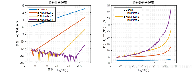
当光滑性足够好时,Richardson外推迭代理论上可以达到任意精度。
给定
f
′
(
x
0
)
f'({{x}_{0}})
f ′ ( x 0 )
f
′
(
x
n
)
f'({{x}_{n}})
f ′ ( x n )
f
′
(
x
)
f'(x)
f ′ ( x )
m
i
=
f
′
(
x
i
)
{{m}_{i}}=f'({{x}_{i}})
m i = f ′ ( x i )
m
i
=
f
(
x
i
+
1
)
−
f
(
x
i
−
1
)
2
h
−
h
2
6
f
′
′
′
(
x
i
)
+
O
(
h
4
)
(1)
{{m}_{i}}=\frac{f({{x}_{i+1}})-f({{x}_{i-1}})}{2h}-\frac{{{h}^{2}}}{6}f'''({{x}_{i}})+O({{h}^{4}})\tag{1}
m i = 2 h f ( x i + 1 ) − f ( x i − 1 ) − 6 h 2 f ′ ′ ′ ( x i ) + O ( h 4 ) ( 1 )
g
g
g
g
(
x
±
h
)
=
g
(
x
)
±
h
g
′
(
x
)
+
h
2
2
g
′
′
(
x
)
±
h
3
6
g
′
′
′
(
x
)
+
O
(
h
4
)
(2)
g(x\pm h)=g(x)\pm hg'(x)+\frac{{{h}^{2}}}{2}g''(x)\pm \frac{{{h}^{3}}}{6}g'''(x)+O({{h}^{4}})\tag{2}
g ( x ± h ) = g ( x ) ± h g ′ ( x ) + 2 h 2 g ′ ′ ( x ) ± 6 h 3 g ′ ′ ′ ( x ) + O ( h 4 ) ( 2 )
g
g
g
g
′
′
(
x
)
=
g
(
x
+
h
)
−
2
g
(
x
)
+
g
(
x
−
h
)
h
2
+
O
(
h
2
)
g''(x)=\frac{g(x+h)-2g(x)+g(x-h)}{{{h}^{2}}}+O({{h}^{2}})
g ′ ′ ( x ) = h 2 g ( x + h ) − 2 g ( x ) + g ( x − h ) + O ( h 2 )
g
=
f
′
g=f'
g = f ′
x
i
{{x}_{i}}
x i
f
′
′
′
f'''
f ′ ′ ′
f
′
′
′
(
x
i
)
=
m
i
+
1
−
2
m
i
+
m
i
−
1
h
2
+
O
(
h
2
)
(3)
f'''({{x}_{i}})=\frac{{{m}_{i+1}}-2{{m}_{i}}+{{m}_{i-1}}}{{{h}^{2}}}+O({{h}^{2}})\tag{3}
f ′ ′ ′ ( x i ) = h 2 m i + 1 − 2 m i + m i − 1 + O ( h 2 ) ( 3 )
f
′
(
x
i
)
f'({{x}_{i}})
f ′ ( x i )
m
i
=
f
(
x
i
+
1
)
−
f
(
x
i
−
1
)
2
h
−
h
2
6
m
i
+
1
−
2
m
i
+
m
i
−
1
h
2
+
O
(
h
4
)
(4)
{{m}_{i}}=\frac{f({{x}_{i+1}})-f({{x}_{i-1}})}{2h}-\frac{{{h}^{2}}}{6}\frac{{{m}_{i+1}}-2{{m}_{i}}+{{m}_{i-1}}}{{{h}^{2}}}+O({{h}^{4}})\tag{4}
m i = 2 h f ( x i + 1 ) − f ( x i − 1 ) − 6 h 2 h 2 m i + 1 − 2 m i + m i − 1 + O ( h 4 ) ( 4 )
m
i
≈
m
i
~
=
f
(
x
i
+
1
)
−
f
(
x
i
−
1
)
2
h
−
h
2
6
m
i
+
1
−
2
m
i
+
m
i
−
1
h
2
{{m}_{i}}\approx \widetilde{{{m}_{i}}}=\frac{f({{x}_{i+1}})-f({{x}_{i-1}})}{2h}-\frac{{{h}^{2}}}{6}\frac{{{m}_{i+1}}-2{{m}_{i}}+{{m}_{i-1}}}{{{h}^{2}}}
m i ≈ m i
= 2 h f ( x i + 1 ) − f ( x i − 1 ) − 6 h 2 h 2 m i + 1 − 2 m i + m i − 1
1
6
(
4
1
1
4
⋱
⋱
⋱
⋱
⋱
4
1
1
4
)
(
m
~
1
m
~
2
⋮
m
~
n
−
2
m
~
n
−
1
)
=
1
2
h
(
f
(
x
2
)
−
f
(
x
0
)
f
(
x
3
)
−
f
(
x
1
)
⋮
f
(
x
n
−
1
)
−
f
(
x
n
−
3
)
f
(
x
n
)
−
f
(
x
n
−
2
)
)
−
1
6
(
m
0
0
⋮
0
m
n
)
\frac{1}{6}\left( \begin{matrix} 4 & 1 & {} & {} & {} \\ 1 & 4 & \ddots & {} & {} \\ {} & \ddots & \ddots & \ddots & {} \\ {} & {} & \ddots & 4 & 1 \\ {} & {} & {} & 1 & 4 \\ \end{matrix} \right)\left( \begin{matrix} {{\widetilde{m}}_{1}} \\ {{\widetilde{m}}_{2}} \\ \vdots \\ {{\widetilde{m}}_{n-2}} \\ {{\widetilde{m}}_{n-1}} \\ \end{matrix} \right)=\frac{\text{1}}{2h}\left( \begin{matrix} f({{x}_{2}})-f({{x}_{0}}) \\ f({{x}_{3}})-f({{x}_{1}}) \\ \vdots \\ f({{x}_{n-1}})-f({{x}_{n-3}}) \\ f({{x}_{n}})-f({{x}_{n-2}}) \\ \end{matrix} \right)-\frac{1}{6}\left( \begin{matrix} {{m}_{0}} \\ 0 \\ \vdots \\ 0 \\ {{m}_{n}} \\ \end{matrix} \right)
6 1 ⎝ ⎜ ⎜ ⎜ ⎜ ⎛ 4 1 1 4 ⋱ ⋱ ⋱ ⋱ ⋱ 4 1 1 4 ⎠ ⎟ ⎟ ⎟ ⎟ ⎞ ⎝ ⎜ ⎜ ⎜ ⎜ ⎜ ⎛ m
1 m
2 ⋮ m
n − 2 m
n − 1 ⎠ ⎟ ⎟ ⎟ ⎟ ⎟ ⎞ = 2 h 1 ⎝ ⎜ ⎜ ⎜ ⎜ ⎜ ⎛ f ( x 2 ) − f ( x 0 ) f ( x 3 ) − f ( x 1 ) ⋮ f ( x n − 1 ) − f ( x n − 3 ) f ( x n ) − f ( x n − 2 ) ⎠ ⎟ ⎟ ⎟ ⎟ ⎟ ⎞ − 6 1 ⎝ ⎜ ⎜ ⎜ ⎜ ⎜ ⎛ m 0 0 ⋮ 0 m n ⎠ ⎟ ⎟ ⎟ ⎟ ⎟ ⎞
O
(
n
)
O(n)
O ( n )
f
(
x
)
=
e
x
;
x
=
1
f(x)={{e}^{x}};x=1
f ( x ) = e x ; x = 1
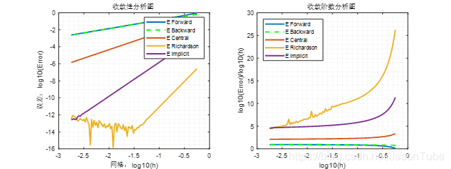
上图是五种方法在没有测量误差的前提下得出的。从左图可知五种方法的收敛性都是满足的,随着网格尺度
h
h
h
上图是在没有测量误差的前提下,使用Richardson方法进行若干次外推和中心差分格式得出的。从图中可知Richardson外推每进行一次迭代收敛阶大约上升两阶,同时可以观察到相同的初始网格尺度
h
h
h
f
(
x
)
=
sin
x
;
x
=
1
f(x)=\sin x;x=1
f ( x ) = sin x ; x = 1
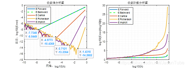
上图是五种方法在没有测量误差的前提下得出的,与算例1中相比较得到的结论是相同的。在将网格进一步加密以后,得到如下图:
从上图可知,随着网格的加密,受舍入误差的影响逐渐明显,最终所有方法都在某一点后不再继续收敛。
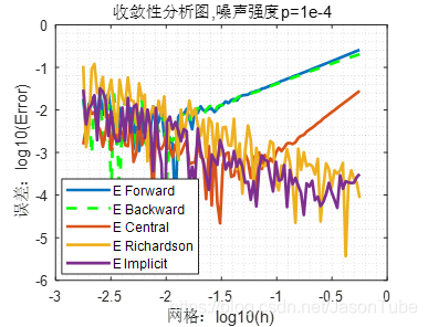
f
(
x
)
=
sin
x
;
x
=
1
f(x)=\sin x;x=1
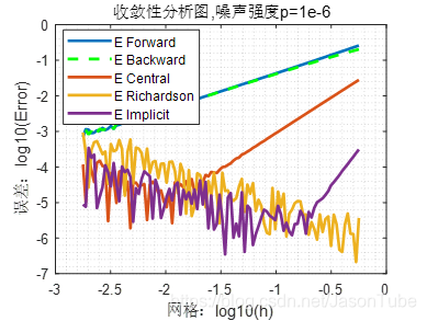
f ( x ) = sin x ; x = 1
从上两图可见,在存在噪声时,随着网格的加密,所有方法都会表现出不适定性,而且随着噪声强度
p
p
p
h
h
h
五种计算方法在以上三个算例中的表现与理论结果基本相符,其中向前差分、向后差分是一阶收敛的,中心差分是二阶收敛的,Richardson外推与中心差分结合后是
2
k
+
2
2k+2
2 k + 2
k
k
k 。
在对数值微分不适定性的观察中,舍入误差的影响随着网格尺寸
h
h
h
h
h
h
从个人的理解中,笔者认为舍入误差和噪声对结果的影响在计算的初始阶段有着相似的特性,都是给精确值加上了一个小的误差
δ
\delta
δ
∣
f
δ
(
x
)
−
f
(
x
)
∣
≤
δ
\left| {{f}^{\delta }}(x)-f(x) \right|\le \delta
∣ ∣ f δ ( x ) − f ( x ) ∣ ∣ ≤ δ
∣
f
δ
(
x
0
+
h
)
−
f
δ
(
x
0
)
h
−
f
′
(
x
0
)
∣
\left| \frac{{{f}^{\delta }}({{x}_{0}}+h)-{{f}^{\delta }}({{x}_{0}})}{h}-f'({{x}_{0}}) \right|
∣ ∣ ∣ ∣ h f δ ( x 0 + h ) − f δ ( x 0 ) − f ′ ( x 0 ) ∣ ∣ ∣ ∣
=
∣
f
δ
(
x
0
+
h
)
−
f
δ
(
x
0
)
h
−
f
(
x
0
+
h
)
−
f
(
x
0
)
h
+
f
(
x
0
+
h
)
−
f
(
x
0
)
h
−
f
′
(
x
0
)
∣
=\left| \frac{{{f}^{\delta }}({{x}_{0}}+h)-{{f}^{\delta }}({{x}_{0}})}{h}-\frac{f({{x}_{0}}+h)-f({{x}_{0}})}{h}+\frac{f({{x}_{0}}+h)-f({{x}_{0}})}{h}-f'({{x}_{0}}) \right|
= ∣ ∣ ∣ ∣ h f δ ( x 0 + h ) − f δ ( x 0 ) − h f ( x 0 + h ) − f ( x 0 ) + h f ( x 0 + h ) − f ( x 0 ) − f ′ ( x 0 ) ∣ ∣ ∣ ∣
≤
c
h
+
2
δ
h
\le ch+\frac{2\delta }{h}
≤ c h + h 2 δ
∣
f
δ
(
x
0
+
h
)
−
f
δ
(
x
0
−
h
)
2
h
−
f
′
(
x
0
)
∣
\left| \frac{{{f}^{\delta }}({{x}_{0}}+h)-{{f}^{\delta }}({{x}_{0}}-h)}{2h}-f'({{x}_{0}}) \right|
∣ ∣ ∣ ∣ 2 h f δ ( x 0 + h ) − f δ ( x 0 − h ) − f ′ ( x 0 ) ∣ ∣ ∣ ∣
=
∣
f
δ
(
x
0
+
h
)
−
f
δ
(
x
0
−
h
)
2
h
−
f
(
x
0
+
h
)
−
f
(
x
0
−
h
)
2
h
+
f
(
x
0
+
h
)
−
f
(
x
0
−
h
)
2
h
−
f
′
(
x
0
)
∣
=\left| \frac{{{f}^{\delta }}({{x}_{0}}+h)-{{f}^{\delta }}({{x}_{0}}-h)}{2h}-\frac{f({{x}_{0}}+h)-f({{x}_{0}}-h)}{2h}+\frac{f({{x}_{0}}+h)-f({{x}_{0}}-h)}{2h}-f'({{x}_{0}}) \right|
= ∣ ∣ ∣ ∣ 2 h f δ ( x 0 + h ) − f δ ( x 0 − h ) − 2 h f ( x 0 + h ) − f ( x 0 − h ) + 2 h f ( x 0 + h ) − f ( x 0 − h ) − f ′ ( x 0 ) ∣ ∣ ∣ ∣
≤
c
h
2
+
δ
h
\le c{{h}^{2}}+\frac{\delta }{h}
≤ c h 2 + h δ
故可知在存在一个小的误差
δ
\delta
δ ,由于Richardson外推在第一层使用了中心差分,且在迭代中要不断将网格继续剖分,同时还有外推累积的误差,故Richardson外推法也会在网格尺度减小到某个值后误差会增大,不再继续收敛,而且这种现象出现的比前面几种低阶格式更早 。
∣
f
′
(
x
0
)
~
−
f
′
(
x
0
)
∣
≤
O
(
h
n
+
δ
h
)
;
n
>
1
\left| \widetilde{f'({{x}_{0}})}-f'({{x}_{0}}) \right|\le O({{h}^{n}}+\frac{\delta }{h});n>1
∣ ∣ ∣ f ′ ( x 0 )
− f ′ ( x 0 ) ∣ ∣ ∣ ≤ O ( h n + h δ ) ; n > 1
O
(
δ
h
)
O(\frac{\delta }{h})
O ( h δ )
f
f
f
h
h
h
O
(
h
n
)
O({{h}^{n}})
O ( h n )
m
i
=
f
(
x
i
+
1
)
−
f
(
x
i
−
1
)
2
h
−
h
2
6
m
i
+
1
−
2
m
i
+
m
i
−
1
h
2
+
O
(
h
4
)
{{m}_{i}}=\frac{f({{x}_{i+1}})-f({{x}_{i-1}})}{2h}-\frac{{{h}^{2}}}{6}\frac{{{m}_{i+1}}-2{{m}_{i}}+{{m}_{i-1}}}{{{h}^{2}}}+O({{h}^{4}})
m i = 2 h f ( x i + 1 ) − f ( x i − 1 ) − 6 h 2 h 2 m i + 1 − 2 m i + m i − 1 + O ( h 4 ) 隐式方法应该也具有不适定性,即在有一个小误差存在时,网格尺度不能无限小,在达到某个值后继续减小误差反而会增大 ,以上的分析与实验结论也基本相符。
接下来是皆大欢喜的MATLAB代码环节 ~
function main
%%
clear;clc;close all;
%%
%初始化
h = 10.^linspace(-0.25,-2.75);
L = length(h);
x0 = 1;%求导点
f=@func;%测试函数
E_Forward = zeros(1,L);
E_Backward = zeros(1,L);
E_Central = zeros(1,L);
E_Richardson = zeros(1,L);
E_Implicit = zeros(1,L);
%%
%计算误差
syms x,y=f(x);
dfunc=diff(y);
for i = 1:L
    Exact_solution=subs(dfunc,x,x0);
    E_Forward(i) = abs(forward(f,x0,h(i)) - Exact_solution);
    E_Backward(i) = abs(backward(f,x0,h(i)) - Exact_solution);
    E_Central(i) = abs(central(f,x0,h(i)) - Exact_solution);
    E_Richardson(i) = abs(richardson(f,x0,h(i),3) - Exact_solution);
    E_Implicit(i) = abs(implicit(f,x0,h(i),20) - Exact_solution);
end
%%
%绘图:log scale(这很重要)
figure;
subplot(1,2,1);
plot(log10(h),log10(E_Forward),'LineWidth',2);hold on;
plot(log10(h),log10(E_Backward),'--g','LineWidth',2);hold on;
plot(log10(h),log10(E_Central),'LineWidth',2);hold on;
plot(log10(h),log10(E_Richardson),'LineWidth',2);hold on;
plot(log10(h),log10(E_Implicit),'LineWidth',2);
legend("E Forward","E Backward","E Central","E Richardson","E Implicit");
title("收敛性分析图")
xlabel("网格:log10(h)")
ylabel("误差:log10(Error)")
grid minor
%%
end

function f = func(x)
%测试函数
%f = exp(x);%x=1
f = sin(x);%x=1
%f = x^(x^x);%x=0.0001
end
function df = forward(f,x0,h)
%向前差分
df = (f(x0+h)-f(x0)) / h;
end
function df = backward(f,x0,h)
%向后差分
df = (f(x0)-f(x0-h)) / h;
end
function df = central(f,x0,h)
%中心差分
df = (f(x0+h)-f(x0-h)) / (2*h);
end
function df = richardson(f,x0,h,N)
%中心差分+Richarson外推,N为外推层数,第一层为中心差分
df_tmp = zeros(1,N);
for i = 1:N
    df_tmp(i) = central(f,x0,2*h*0.5^i);
end
%disp("Richarson外推过程:")
%disp(df_tmp)
for i = 1:N
    j = N-i;
    df_tmp(1:j) = (df_tmp(2:j+1)*4^i - df_tmp(1:j)) / (4^i-1);
    %disp(df_tmp(1:j))
end
df = df_tmp(1);
end
function df=implicit(f,x0,h,N)
%隐格式,在x0附近计算2N+1个点的微分,默认最远两端点导数为已知
n=2*N+1;
F=zeros(n,1);
x1=x0-N*h;
for i=1:n
    F(i)=f(x1+i*h)-f(x1+(i-2)*h);
end
F=F/(2*h);
%求已知点导数
syms x,y=f(x);
dfun=diff(y);
F(1)=F(1)-subs(dfun,x,x1)/6;
F(n)=F(n)-subs(dfun,x,x0+N*h)/6;
%追赶法求解三对角系数矩阵的线性方程组
M=crout(2*ones(1,n)/3,ones(1,n-1)/6,ones(1,n-1)/6,F);
df=M(N+1);
end
function x=crout(a,c,d,b)
%追赶法 a:主对角线 c、d:次对角线
n=length(a);
n1=length(c);
n2=length(d);
p=1:n;
q=1:n-1;
x=1:n;
y=1:n;
p(1)=a(1);
for i=1:n-1
    q(i)=c(i)/p(i);
    p(i+1)=a(i+1)-d(i)*q(i);
end
y(1)=b(1)/p(1);
for i=2:n
    y(i)=(b(i)-d(i-1)*y(i-1))/p(i);
end
x(n)=y(n);
for i=(n-1):-1:1
    x(i)=y(i)-q(i)*x(i+1);
end
end