机器学习——线性回归（数学原理推导+Python代码实现+模型评估+实验分析）

机器学习——线性回归

（一）线性回归原理推导
（二）线性回归代码实现
（三）模型评估方法
（四）线性回归实验分析

（一）线性回归原理推导

线性回归：用一条直线较为精确地描述数据之间的关系。这样当出现新的数据的时候，就能够预测出一个简单的值。

1.1 模型描述

线性回归按变量数量的多少可以分为：一元线性回归（简单线性回归）和多元线性回归。

一元线性回归（有一个自变量），模型可以表示如下：
$y=\theta _{0}+\theta _{1}x_{1}+\varepsilon$

$x$ ：自变量（数据）
$y$ ：因变量（标签）
$\theta _{0}$ ：截距
$\theta _{1}$ ：变量回归系数
$\varepsilon$ : 误差项的随机变量

$\theta _{0}+\theta _{1}x$ ：反映了由于x的变化而引起的y的线性变化。
$\varepsilon$ ：反映了除了x和y之间的线性关系之外的随机因素对y的影响。也可以说是真实值和预测值之间的误差。希望这个误差项越小越好，并且接近于0。

误差 $\varepsilon$ 是独立并且具有相同的分布，服从均值为0，方差为 $\theta ^{2}$ 的高斯分布。(没有数据可以100%服从这个分布，但不代表这个事情做不了，数学原理是推导理论的支撑，实际上，数据来源于生活，服务于生活，就足够了，没有绝对正确的东西，我们得到的是一个近似的，最优的结果)

多元线性回归（有多个自变量），模型可以表示如下：
$y=\theta _{0}+\theta _{1}x_{1}+\theta _{2}x_{2}+...+\theta _{k}x_{k}+\varepsilon$

$h_{\theta }(x)=\theta _{0}+\theta _{1}x_{1}+\theta _{2}x_{2}+...+\theta _{k}x_{k}$ ：拟合的平面（如图，平面方程估计的结果就是预测值，红色的点是真实值）

$\theta _{0}$ ：偏置项（在训练过程中，使模型能够更精准做的微调）
$\theta _{1}，\theta _{2}...$ ：权重项（核心影响因素）

注意：数据x是一个矩阵，行代表样本，列代表特征，所有对数据的操作，都是对矩阵的操作。而 $\theta _{0}+\theta _{1}x_{1}+\theta _{2}x_{2}+...+\theta _{k}x_{k}$ 多了 $\theta _{0}$ ，由于 $\theta _{0}$ 的存在，没办法转换为矩阵，如果找到 $x _{0}$ 和 $\theta _{0}$ 组合在一起就可以转换为矩阵形式，而 $x_{1}$ ， $x_{2}$ 都是实际存在的特征，可以创建新的一列 $x _{0}$ ，值全为1，因为1乘以一个数等于它本身。

现在就可以转换为一种矩阵形式。整合： $h_{\theta }(x)=\sum_{i=0}^{n}\theta _{i}x_{i}=\theta ^{T}x$

对于每个样本： $y^{(i)}=\theta ^{T}x^{(i)}+\varepsilon ^{(i)}$

误差服从高斯分布： $p(\varepsilon ^{(i)})=\frac{1}{\sqrt{2\pi\sigma}}exp(-\frac{(\varepsilon^{(i)})^{2}}{2\sigma^{2}})$

整合： $p(y^{(i)}|x^{(i)};\theta)=\frac{1}{\sqrt{2\pi\sigma}}exp(-\frac{(y^{(i)}-\theta ^{T}x^{(i)})^{2}}{2\sigma^{2}})$

似然函数： $L(\theta)=\prod_{i=1}^{m}p(y^{(i)}|x^{(i)};\theta)=\prod_{i=1}^{m}\frac{1}{\sqrt{2\pi\sigma}}exp(-\frac{(y^{(i)}-\theta ^{T}x^{(i)})^{2}}{2\sigma^{2}})$

解释：什么样的参数跟我们的数据组合后恰好是真实值。

对数函数： $logL(\theta)=log\prod_{i=1}^{m}\frac{1}{\sqrt{2\pi\sigma}}exp(-\frac{(y^{(i)}-\theta ^{T}x^{(i)})^{2}}{2\sigma^{2}})$

解释：乘法难解，加法就容易多了，对数里面的乘法可以转换为加法。转换完之后，求解的结果变了，但是我们并不关心 $L(\theta)$ ， $logL(\theta)$ 是什么，我们要求的是极值点 $\theta$ ，而不是极值。

展开化简：
$log\prod_{i=1}^{m}\frac{1}{\sqrt{2\pi\sigma}}exp(-\frac{(y^{(i)}-\theta ^{T}x^{(i)})^{2}}{2\sigma^{2}})$

= $\sum_{i=1}^{m}log\frac{1}{\sqrt{2\pi\sigma}}exp(-\frac{(y^{(i)}-\theta ^{T}x^{(i)})^{2}}{2\sigma^{2}})$

= $mlog\frac{1}{\sqrt{2\pi\sigma}}-\frac{1}{\sigma^{2}}\cdot \frac{1}{2}\sum_{i=1}^{m}(y^{(i)}-\theta ^{T}x^{(i)})^{2}$

目标：让似然函数（对数变换后也一样）越大越好，由于 $mlog\frac{1}{\sqrt{2\pi\sigma}}$ 是常数，则代价函数越小越好。

代价函数： $J(\theta)=\frac{1}{2}\sum_{i=1}^{m}(y^{(i)}-\theta ^{T}x^{(i)})^{2}$ （最小二乘法）

x不是一个数，而是一个矩阵，对于矩阵来说，平方项等于转置乘以自身。

$J(\theta)=\frac{1}{2}\sum_{i=1}^{m}(\theta ^{T}x^{(i)}-y^{(i)})^{2}=\frac{1}{2}(X\theta-y)^{T}(X\theta -y)$

求偏导：
$\triangledown _{\theta}J(\theta)=\triangledown _{\theta}(\frac{1}{2}(X\theta-y)^{T}(X\theta -y)$

$=\triangledown _{\theta}(\frac{1}{2}(\theta ^{T}X^{T}-y^{T})(X\theta -y)$

$=\triangledown _{\theta}(\frac{1}{2}(\theta ^{T}X^{T}X\theta-\theta ^{T}X\theta y-y^{T}X\theta +y^{T}y))$

$=\frac{1}{2}(2X^{T}X\theta-X^{T}y-(y^{T}X)^{T})$

$=X^{T}X\theta -X^{T}y$

偏导等于0： $\theta =(X^{T}X)^{-1}X^{T}y$

1.2 梯度下降

在机器学习中反复出现的一个问题：好的泛化需要大的训练集，但大的训练集的计算代价也大。一般来说，代价函数越小，就也意味着模型拟合得越好。所以梯度下降就是帮助我们最小化代价函数、损失函数的常用方法。

梯度下降背后的思想是：开始时我们随机选择一个参数的组合(?0,?1,…,??)，计算代
价函数，然后我们寻找下一个能让代价函数值下降最多的参数组合。我们持续这么做直到到
到一个局部最小值（local minimum），因为我们并没有尝试完所有的参数组合，所以不能确定我们得到的局部最小值是否便是全局最小值（global minimum），选择不同的初始参数组合，可能会找到不同的局部最小值。

想象一下你正站立在山的这一点上，站立在你想象的公园这座红色山上，在梯度下降算
法中，我们要做的就是旋转 360 度，看看我们的周围，并问自己要在某个方向上，用小碎步
尽快下山。这些小碎步需要朝什么方向？如果我们站在山坡上的这一点，你看一下周围，你
会发现最佳的下山方向，你再看看周围，然后再一次想想，我应该从什么方向迈着小碎步下
山？然后你按照自己的判断又迈出一步，重复上面的步骤，从这个新的点，你环顾四周，并
决定从什么方向将会最快下山，然后又迈进了一小步，并依此类推，直到你接近局部最低点
的位置。

目标函数（代价函数）：

$J(\theta_{0},\theta_{1})=\frac{1}{2m}\sum_{i=1}^{m}(h_{\theta}(x^{(i)})-y^{(i)})^{2}$

批量梯度下降：批量梯度下降法是最原始的形式，它是指在每一次迭代时使用所有样本来进行梯度的更新。
$\theta j:=\theta j-\alpha \frac{\partial J(\theta)}{\partial \theta j}$

$\frac{ \partial J(\theta)}{\partial \theta _{j}}=\frac{1}{m}\sum_{i=1}^{m}(h_{\theta}(x^{(i)})-y^{(i)})x_{j}^{i}$

$\theta_{j}:=\theta_{j}-\frac{1}{m}\alpha\sum_{i=1}^{m}(h_{\theta}(x^{(i)})-y^{(i)})x_{j}^{i}$

(由全数据集确定的方向能够更好地代表样本总体，从而更准确地朝向极值所在的方向。一次迭代是对所有样本进行计算，此时利用矩阵进行操作，实现了并行。当目标函数为凸函数时，容易得到最优解，但是由于每次考虑所有样本，速度很慢）

随机梯度下降：每次迭代使用一个样本来对参数进行更新。

$\theta_{j}:=\theta_{j}-\alpha(h_{\theta}(x^{(i)})-y^{(i)})x_{j}^{i}$

(每次找一个样本，迭代速度快，但不一定每次都朝着收敛的方向，不易于并行实现。）

小批量梯度下降：每次迭代使用batch_size个样本来对参数进行更新。这里假设 batchsize=10 ：

$\theta_{j}:=\theta_{j}-\alpha\frac{1}{10}\sum_{k=i}^{i+9}(h_{\theta}(x^{(k)})-y^{(k)})x_{j}^{(k)}$

(通过矩阵运算，每次在一个batch上优化神经网络参数并不会比单个数据慢太多。使用一个batch可以大大减小收敛所需要的迭代次数，同时可以使收敛到的结果更加接近梯度下降的效果。可实现并行化。)

$\alpha$ 是学习率（learning rate），它决定了我们沿着能让代价函数下降程度最大的方向向下迈出的步子有多大。

如果 $\alpha$ 太小的话，可能会很慢，因为它会一点点挪动，它会需要很多步才能到达全局最低点。
如果 $\alpha$ 太大，那么梯度下降法可能会越过最低点，甚至可能无法收敛，下一次迭代又移动了一大步，越过一次，又越过一次，一次次越过最低点，直到你发现实际上离最低点越来远，所以，如果?太大，它会导致无法收敛，甚至发散。

（二）线性回归代码实现

线性回归算法，实现对数据的预处理操作，梯度下降优化，损失与预测：

# -*- coding: utf-8 -*-
import numpy as np
from utils.features import prepare_for_training

class LinearRegression:

    def __init__(self,data,labels,polynomial_degree = 0,sinusoid_degree = 0,normalize_data=True):
        """
        1.对数据进行预处理操作
        2.先得到所有的特征个数
        3.初始化参数矩阵
        """
        (data_processed,
         features_mean, 
         features_deviation)  = prepare_for_training(data, polynomial_degree, sinusoid_degree,normalize_data=True)
         
        self.data = data_processed
        self.labels = labels
        self.features_mean = features_mean
        self.features_deviation = features_deviation
        self.polynomial_degree = polynomial_degree
        self.sinusoid_degree = sinusoid_degree
        self.normalize_data = normalize_data
        
        num_features = self.data.shape[1]  #表示有多少列
        self.theta = np.zeros((num_features,1))
         #训练函数
    def train(self,alpha,num_iterations = 500):
         #训练模块，执行梯度下降
        cost_history = self.gradient_descent(alpha,num_iterations)
        return self.theta,cost_history
        
    def gradient_descent(self,alpha,num_iterations):
        #实际迭代模块，会迭代num_iterations次
        cost_history = []   
        #每次损失的变化，记为一个list
        for _ in range(num_iterations):
            self.gradient_step(alpha)
            cost_history.append(self.cost_function(self.data,self.labels))
        return cost_history   #返回损失值
             
    def gradient_step(self,alpha):    
        #梯度下降参数更新计算方法，注意是矩阵运算
        num_examples = self.data.shape[0]  #样本个数
        prediction = LinearRegression.hypothesis(self.data,self.theta)  #预测值
        delta = prediction - self.labels  #预测值减真实值
        theta = self.theta
        theta = theta - alpha*(1/num_examples)*(np.dot(delta.T,self.data)).T  #矩阵计算，不用循环
        self.theta = theta   #更新theta
        
        
    def cost_function(self,data,labels):
        #损失计算方法
        num_examples = data.shape[0]
        delta = LinearRegression.hypothesis(self.data,self.theta) - labels   #预测值-labels
        cost = (1/2)*np.dot(delta.T,delta)/num_examples   #损失函数
        return cost[0][0]
        
    @staticmethod
    def hypothesis(data,theta):   
        predictions = np.dot(data,theta)
        return predictions
        
    def get_cost(self,data,labels):  
        data_processed = prepare_for_training(data,
         self.polynomial_degree,
         self.sinusoid_degree,
         self.normalize_data
         )[0]  #只要数据
        return self.cost_function(data_processed,labels)

    def predict(self,data):
         # 用训练的参数模型，与预测得到回归值结果
        data_processed = prepare_for_training(data,
         self.polynomial_degree,
         self.sinusoid_degree,
         self.normalize_data
         )[0]
         
        predictions = LinearRegression.hypothesis(data_processed,self.theta    
        return predictions

把上面的算法应用到实际应用中：
先做单变量线性回归，只选择一个特征，对应一个 $\theta$ 参数，画出原始数据的散点图：

# -*- coding: utf-8 -*-
import numpy as np
import pandas as pd
import matplotlib.pyplot as plt
from linear_regression import LinearRegression

data = pd.read_csv('../data/world-happiness-report-2017.csv')

# 得到训练和测试数据
train_data = data.sample(frac = 0.8)
test_data = data.drop(train_data.index)   #把训练数据去掉

input_param_name = 'Economy..GDP.per.Capita.'
output_param_name = 'Happiness.Score'

x_train = train_data[[input_param_name]].values
y_train = train_data[[output_param_name]].values

x_test = test_data[input_param_name].values
y_test = test_data[output_param_name].values

plt.scatter(x_train,y_train,label='Train data')
plt.scatter(x_test,y_test,label='test data')
plt.xlabel(input_param_name)
plt.ylabel(output_param_name)
plt.title('Happy')
plt.legend()
plt.show()

接下来训练线性回归模型：

num_iterations = 500    #迭代500次
learning_rate = 0.01    #学习率

linear_regression = LinearRegression(x_train,y_train) #初始化
(theta,cost_history) = linear_regression.train(learning_rate,num_iterations)

print '开始时的损失：',cost_history[0]
print '训练后的损失：',cost_history[-1]

plt.plot(range(num_iterations),cost_history)
plt.xlabel('Iter')   #迭代次数
plt.ylabel('cost')   #损失
plt.title('GD')
plt.show()

最后测试，得到线性回归方程：

predictions_num = 100   #测试数量
x_predictions = np.linspace(x_train.min(),x_train.max(),predictions_num).reshape(predictions_num,1)
y_predictions = linear_regression.predict(x_predictions)   #通过x预测y
 
plt.scatter(x_train,y_train,label='Train data')
plt.scatter(x_test,y_test,label='test data')
plt.plot(x_predictions,y_predictions,'r',label = 'Prediction')
plt.xlabel(input_param_name)
plt.ylabel(output_param_name)
plt.title('Happy')
plt.legend()
plt.show()

红色的线就是最终实际预测的结果。

下面对应多特征回归，画出原始数据的散点图：

import numpy as np
import pandas as pd
import matplotlib.pyplot as plt
import plotly    #绘图
import plotly.graph_objs as go

plotly.offline.init_notebook_mode()
from linear_regression import LinearRegression

data = pd.read_csv('../data/world-happiness-report-2017.csv')

train_data = data.sample(frac=0.8)
test_data = data.drop(train_data.index)

input_param_name_1 = 'Economy..GDP.per.Capita.'
input_param_name_2 = 'Freedom'
output_param_name = 'Happiness.Score'


x_train = train_data[[input_param_name_1, input_param_name_2]].values
y_train = train_data[[output_param_name]].values

x_test = test_data[[input_param_name_1, input_param_name_2]].values
y_test = test_data[[output_param_name]].values

# 使用训练数据集绘图。
plot_training_trace = go.Scatter3d(
    x=x_train[:, 0].flatten(),
    y=x_train[:, 1].flatten(),
    z=y_train.flatten(),
    name='Training Set',
    mode='markers',
    marker={
        'size': 10,
        'opacity': 1,
        'line': {
            'color': 'rgb(255, 255, 255)',
            'width': 1
        },
    }
)

# 使用测试数据集绘图。
plot_test_trace = go.Scatter3d(
    x=x_test[:, 0].flatten(),
    y=x_test[:, 1].flatten(),
    z=y_test.flatten(),
    name='Test Set',
    mode='markers',
    marker={
        'size': 10,
        'opacity': 1,
        'line': {
            'color': 'rgb(255, 255, 255)',
            'width': 1
        },
    }
)


plot_layout = go.Layout(
    title='Date Sets',
    scene={
        'xaxis': {'title': input_param_name_1},
        'yaxis': {'title': input_param_name_2},
        'zaxis': {'title': output_param_name} 
    },
    margin={'l': 0, 'r': 0, 'b': 0, 't': 0}
)
plot_data = [plot_training_trace, plot_test_trace]

plot_figure = go.Figure(data=plot_data, layout=plot_layout)

plotly.offline.plot(plot_figure)   #在网页中打开界面

接下来训练模型：


num_iterations = 500  
learning_rate = 0.01  
polynomial_degree = 0  
sinusoid_degree = 0  

linear_regression = LinearRegression(x_train, y_train, polynomial_degree, sinusoid_degree)

(theta, cost_history) = linear_regression.train(
    learning_rate,
    num_iterations
)

print('开始损失',cost_history[0])
print('结束损失',cost_history[-1])

plt.plot(range(num_iterations), cost_history)
plt.xlabel('Iterations')
plt.ylabel('Cost')
plt.title('Gradient Descent Progress')
plt.show()

观察发现：开始损失都是相似的，但结束损失有两个特征值时比一个特征值时损失值更低一些。

最后测试：

predictions_num = 10

x_min = x_train[:, 0].min();
x_max = x_train[:, 0].max();

y_min = x_train[:, 1].min();
y_max = x_train[:, 1].max();


x_axis = np.linspace(x_min, x_max, predictions_num)
y_axis = np.linspace(y_min, y_max, predictions_num)


x_predictions = np.zeros((predictions_num * predictions_num, 1))
y_predictions = np.zeros((predictions_num * predictions_num, 1))

x_y_index = 0
for x_index, x_value in enumerate(x_axis):
    for y_index, y_value in enumerate(y_axis):
        x_predictions[x_y_index] = x_value
        y_predictions[x_y_index] = y_value
        x_y_index += 1

z_predictions = linear_regression.predict(np.hstack((x_predictions, y_predictions)))

plot_predictions_trace = go.Scatter3d(
    x=x_predictions.flatten(),
    y=y_predictions.flatten(),
    z=z_predictions.flatten(),
    name='Prediction Plane',
    mode='markers',
    marker={
        'size': 1,
    },
    opacity=0.8,
    surfaceaxis=2, 
)

plot_data = [plot_training_trace, plot_test_trace, plot_predictions_trace]
plot_figure = go.Figure(data=plot_data, layout=plot_layout)
plotly.offline.plot(plot_figure)

蓝色的面就是最终得到的结果，相当于回归面，对于不同的x，y值，都分别得到对应的z值。

非线性回归：

import numpy as np
import pandas as pd
import matplotlib.pyplot as plt

from linear_regression import LinearRegression

data = pd.read_csv('../data/non-linear-regression-x-y.csv')

x = data['x'].values.reshape((data.shape[0], 1))
y = data['y'].values.reshape((data.shape[0], 1))

data.head(10)

plt.plot(x, y)
plt.show()

训练模型

num_iterations = 50000    #迭代次数
learning_rate = 0.02  
polynomial_degree = 15  
sinusoid_degree = 15  
normalize_data = True  

linear_regression = LinearRegression(x, y, polynomial_degree, sinusoid_degree, normalize_data)

(theta, cost_history) = linear_regression.train(
    learning_rate,
    num_iterations
)

print('开始损失: {:.2f}'.format(cost_history[0]))
print('结束损失: {:.2f}'.format(cost_history[-1]))

theta_table = pd.DataFrame({'Model Parameters': theta.flatten()})


plt.plot(range(num_iterations), cost_history)
plt.xlabel('Iterations')
plt.ylabel('Cost')
plt.title('Gradient Descent Progress')
plt.show()

观察到在很少的次数就已经达到比较好的效果了，但是虽然左下角看着比较接近0，其实还是一个比较大的结果，大概是35，有一个问题就是会过拟合，因为模型越复杂，测试集得到的结果问题越大。

测试：

predictions_num = 1000
x_predictions = np.linspace(x.min(), x.max(), predictions_num).reshape(predictions_num, 1);
y_predictions = linear_regression.predict(x_predictions)

plt.scatter(x, y, label='Training Dataset')
plt.plot(x_predictions, y_predictions, 'r', label='Prediction')
plt.show()

蓝色线是数据，红色线是回归方程曲线。

（三）模型评估方法

3.1 数据集切分

import numpy as np
import os
%matplotlib inline
import matplotlib
import matplotlib.pyplot as plt
plt.rcParams['axes.labelsize'] = 14   #设置字体大小
plt.rcParams['xtick.labelsize'] = 12
plt.rcParams['ytick.labelsize'] = 12
import warnings
warnings.filterwarnings('ignore')
np.random.seed(42)

from sklearn.datasets import fetch_mldata
mnist = fetch_mldata('MNIST original')   #读取数据集
mnist   #Mnist数据是图像数据，（28,28,1）的灰度图

X, y = mnist["data"], mnist["target"]
X.shape   #数据中一共有70000个样本，每个样本长宽都是28，颜色通道是1，28x28x1=784

(70000, 784)

X_train, X_test, y_train, y_test = X[:60000], X[60000:], y[:60000], y[60000:]  #训练集取前60000个，测试集取后10000个 ，训练集测试集切分是为了建模完之后还要再进行评估，

# 洗牌操作，把数据打乱
import numpy as np

shuffle_index = np.random.permutation(60000)
X_train, y_train = X_train[shuffle_index], y_train[shuffle_index]

shuffle_index  #可以看到数据已经被打乱

array([12628, 37730, 39991, …, 860, 15795, 56422])

3.2 交叉验证的作用

数据集被分为训练集和测试集，训练集是实际训练用到的数据集，把训练中没用过的数据做测试集，一般情况下8:2比较常见，假如有100个数据，训练集80个，测试集20个。训练集做交叉验证，相当于自我调节过程，比如把训练集平均切分成10份，在某一次测试中，拿前九份做训练集，拿第10份当测试集，但是有问题，测试集结果跟选择数据的切分有关，所以这时候就做交叉验证，可以选择拿1到8以及10做训练集，9做测试集，以此类推，这样就做10次验证，取平均结果。

下面就是具体过程图

从代码中演示交叉验证

#建立模型，判断一个数字是5还是不是5
y_train_5 = (y_train==5)
y_test_5 = (y_test==5)

y_train_5[:10]   #查看前10个数据

array([False, False, False, False, False, False, False, False, False,
True])

from sklearn.linear_model import SGDClassifier   #SGD分类器
sgd_clf = SGDClassifier(max_iter=5,random_state=42)   #迭代5次,设置每次随机结果都是一样的
sgd_clf.fit(X_train,y_train_5)

sgd_clf.predict([X[35000]])   #预测第35000个数据是5还是不是5

array([ True])

y[35000]    #实际标签确实等于5

5.0

3.3 交叉验证实验分析

#用sklearn中的cross_val_score函数
m sklearn.model_selection import cross_val_score
cross_val_score(sgd_clf,X_train,y_train_5,cv=3,scoring='accuracy')   #交叉验证做三次,指定准确率作为评估方法

array([0.9502 , 0.96565, 0.96495]) #交叉验证三次的结果


#用sklearn中的StratifiedKFold函数
from sklearn.model_selection import StratifiedKFold
from sklearn.base import clone  #构建模型都是用相同的参数,保证公平,所以用clone 方法

skflods = StratifiedKFold(n_splits=3,random_state=42)
for train_index,test_index in skflods.split(X_train,y_train_5): #数据集和标签都要切分
    clone_clf = clone(sgd_clf)  #克隆一个分类器
    X_train_folds = X_train[train_index]
    y_train_folds = y_train_5[train_index]
    X_test_folds = X_train[test_index]
    y_test_folds = y_train_5[test_index]
    
    clone_clf.fit(X_train_folds,y_train_folds)   #训练
    y_pred = clone_clf.predict(X_test_folds)   #测试数据
    n_correct = sum(y_pred == y_test_folds)  #检查测试结果和实际标签是不是一样的,看下做对多少个
    print(n_correct/len(y_pred))

0.9502
0.96565
0.96495

3.4 混淆矩阵

已知条件:班级总人数100人,其中男生80人,女生20人.
目标: 找出所有的女生
结果: 从班级中选择了50人,其中20人是女生,错误的把30个男生也挑选出来了。

	相关（Relevant），正类	无关（NonRelevant），负类
被检索到	true positives(TP 正类判定为正类，例子中就是正确的判定“这位是女生”)	false positives(FP 负类判定为正类，例子中就是男生判定为女生)
未被检索到	false negatives(FN 正类判定为负类，例子中就是女生判断为男生)	true negatives(TN 负类判定为负类，例子中就是男生判定为男生)

from sklearn.model_selection import cross_val_predict
y_train_pred = cross_val_predict(sgd_clf,X_train,y_train_5,cv=3) #返回样本预测的结果

y_train_pred.shape  #训练集大小是一样的

(60000,)

X_train.shape

(60000, 784)

#sklearn中的confusion_matrix函数得到混淆矩阵
from sklearn.metrics import confusion_matrix
confusion_matrix(y_train_5,y_train_pred)

array([[53272, 1307],
[ 1077, 4344]], dtype=int64)

negative class [[ true negatives , false positives ],
positive class [ false negatives , true positives ]]

1.true negatives: 53,272个数据被正确的分为非5类别
2.false positives：1307张被错误的分为5类别
3.false negatives：1077张错误的分为非5类别
4.true positives： 4344张被正确的分为5类别

一个完美的分类器应该只有true positives 和 true negatives, 即主对角线元素不为0，其余元素为0

3.5 评估指标对比分析

精度： $precision = \frac {TP} {TP + FP}$
召回率： $recall = \frac {TP} {TP + FN}$

from sklearn.metrics import precision_score,recall_score
precision_score(y_train_5,y_train_pred)   #精度

0.7687135020350381

recall_score(y_train_5,y_train_pred)   #召回率

0.801328168234643

将Precision 和 Recall结合到一个称为 $F_1$ score (调和平均数)的指标,调和平均值给予低值更多权重。因此，如果召回和精确度都很高，分类器将获得高 $F_1$ 分数。

$F_1 =$

$2\over {1\over precision}+{1\over recall}$

$=2×precision×recall\over precision+recall$

= $TP\over {TP}+{FN + FP\over 2}$

from sklearn.metrics import f1_score
f1_score(y_train_5,y_train_pred)

0.7846820809248555

3.6 阈值对结果的影响

y_scores = sgd_clf.decision_function([X[35000]])
y_scores        #得分值  算法中都会得到一个得分值，x和权重参数结合在一起得到的是一个得分值而不是一个概率值，根据得分值判断属于哪一类

array([43349.73739616])

t = 50000     #设置阈值,最终分类是不是5可以由自己决定
y_pred = (y_scores > t)
y_pred

array([False])

t = 0     #设置阈值
y_pred = (y_scores > t)
y_pred

array([True])

可以看到精度和recall值在阈值影响下的结果，精度高，recall值就低，精度低，recall值就高。

Scikit-Learn不允许直接设置阈值，但它可以得到决策分数，调用其decision_function()方法，而不是调用分类器的predict()方法，该方法返回每个实例的分数，然后使用想要的阈值根据这些分数进行预测：

y_scores = cross_val_predict(sgd_clf, X_train, y_train_5, cv=3,method="decision_function")

y_scores[:10]   #得分值

array([ -434076.49813641, -1825667.15281624, -767086.76186905,
-482514.55006702, -466416.8082872 , -311904.74603814,
-582112.5580173 , -180811.15850786, -442648.13282116,
-87710.09830358])

from sklearn.metrics import precision_recall_curve
precisions, recalls, thresholds = precision_recall_curve(y_train_5, y_scores)

y_train_5.shape

(60000,)

thresholds.shape   #阈值个数，把所有可能值拿出来做尝试，有300多个重复的

(59698,)

precisions[:10]   #每一个阈值下都有对应的精度和recall值结果

array([0.09080706, 0.09079183, 0.09079335, 0.09079487, 0.09079639,
0.09079792, 0.09079944, 0.09080096, 0.09080248, 0.090804 ])

precisions.shape   #因为一个阈值切成两份，所以比59698多了一个

(59699,)

recalls.shape

(59699,)

def plot_precision_recall_vs_threshold(precisions,recalls,thresholds):
    plt.plot(thresholds,
             precisions[:-1],
            "b--",
            label="Precision")
    
    plt.plot(thresholds,
             recalls[:-1],
            "g-",
            label="Recall")
    plt.xlabel("Threshold",fontsize=16)
    plt.legend(loc="upper left",fontsize=16)
    plt.ylim([0,1])
    
plt.figure(figsize=(8, 4))
plot_precision_recall_vs_threshold(precisions,recalls,thresholds)
plt.xlim([-700000, 700000])
plt.show()

对于不同的阈值，精度和recall值预测的情况：

def plot_precision_vs_recall(precisions, recalls):
    plt.plot(recalls, 
             precisions, 
             "b-", 
             linewidth=2)
    
    plt.xlabel("Recall", fontsize=16)
    plt.ylabel("Precision", fontsize=16)
    plt.axis([0, 1, 0, 1])

plt.figure(figsize=(8, 6))
plot_precision_vs_recall(precisions, recalls)
plt.show()

随着recall值的变化，精度变化的情况：

3.7 ROC 曲线

receiver operating characteristic (ROC) 曲线是二元分类中的常用评估方法。它与精确度/召回曲线非常相似，但ROC曲线不是绘制精确度与召回率，而是绘制true positive rate(TPR) 与false positive rate(FPR)

$TPR = TP / (TP + FN) (Recall)$
$FPR = FP / (FP + TN)$

from sklearn.metrics import roc_curve
fpr, tpr, thresholds = roc_curve(y_train_5, y_scores)

def plot_roc_curve(fpr, tpr, label=None):
    plt.plot(fpr, tpr, linewidth=2, label=label)
    plt.plot([0, 1], [0, 1], 'k--')
    plt.axis([0, 1, 0, 1])
    plt.xlabel('False Positive Rate', fontsize=16)
    plt.ylabel('True Positive Rate', fontsize=16)

plt.figure(figsize=(8, 6))
plot_roc_curve(fpr, tpr)
plt.show()

虚线表示纯随机分类器的ROC曲线; 一个好的分类器尽可能远离该线（朝左上角）

比较分类器的一种方法是测量曲线下面积（AUC）。完美分类器的ROC AUC等于1，而纯随机分类器的ROC AUC等于0.5。 Scikit-Learn提供了计算ROC AUC的函数：

from sklearn.metrics import roc_auc_score
roc_auc_score(y_train_5, y_scores)

0.9624496555967156 #预测结果还是不错的

（四）线性回归实验分析

import numpy as np
import os
%matplotlib inline
import matplotlib
import matplotlib.pyplot as plt
plt.rcParams['axes.labelsize'] = 14
plt.rcParams['xtick.labelsize'] = 12
plt.rcParams['ytick.labelsize'] = 12
import warnings
warnings.filterwarnings('ignore')
np.random.seed(42)

import numpy as np
X = 2*np.random.rand(100,1)    #创建随机数据，100个点
y = 4+ 3*X +np.random.randn(100,1)  #随便构造一个方程 学习

plt.plot(X,y,'b.')
plt.xlabel('X_1')     #数据中只有一个特征
plt.ylabel('y')
plt.axis([0,2,0,15])  #x轴0到2，y轴0到15
plt.show()

4.1 参数直接求解方法

X_b = np.c_[np.ones((100,1)),X]    #在数据集左侧拼上一列1
theta_best = np.linalg.inv(X_b.T.dot(X_b)).dot(X_b.T).dot(y)

theta_best参照公式： $\hat{\theta} =(X^{T}X)^{-1}X^{T}y$

theta_best

array([[4.21509616],
[2.77011339]])

也可以用sklearn实现

from sklearn.linear_model import LinearRegression
lin_reg = LinearRegression()
lin_reg.fit(X,y)
print (lin_reg.coef_)        #权重参数
print (lin_reg.intercept_)   #偏置参数

[[2.77011339]]
[4.21509616]

X_new = np.array([[0],[2]])             #两个数据点
X_new_b = np.c_[np.ones((2,1)),X_new]   #加一列1
y_predict = X_new_b.dot(theta_best)     #用当前数据乘以参数得到实际预测结果
y_predict

array([[4.21509616],
[9.75532293]])

plt.plot(X_new,y_predict,'r--')   #画出两个点得到的一条线
plt.plot(X,y,'b.')
plt.axis([0,2,0,15])
plt.show()

可以看到只要有数据x,y就能得到回归方程，但是观察公式 $\hat{\theta} =(X^{T}X)^{-1}X^{T}y$ ，转置还好求解，但是矩阵的逆不是所有情况都能求出来的，机器学习的思想也不在于此，应该是去学习，而不是拿到数据直接求解，下面会解释梯度下降怎么解决问题的。

4.2 预处理对结果的影响

当步长太小时：

当步长太大时：

学习率应当尽可能小，随着迭代的进行应当越来越小。

4.3 梯度下降模块

批量梯度下降

$\bigtriangledown\theta MSE(\theta)=\frac{2}{m}X^{T}\cdot(X\cdot\theta-y)$

eta = 0.1   #学习率
n_iterations = 1000   #迭代次数
m = 100  #样本个数
theta = np.random.randn(2,1)   #随机初始化 
for iteration in range(n_iterations):
    gradients = 2/m* X_b.T.dot(X_b.dot(theta)-y)   #参照上面公式
    theta = theta - eta*gradients   #梯度更新

theta    #有两个theta，跟直接算结果差不多

array([[4.21509616], #偏执参数
[2.77011339]]) #权重参数

X_new_b.dot(theta)   #得到最终预测出来的结果值

array([[4.21509616],
[9.75532293]])

随机梯度下降

theta_path_sgd=[]
m = len(X_b)    #计算所有样本
np.random.seed(42)   #指定随机种子，随机选择相同theta，theta不变，数据不变，结果不变
n_epochs = 50

t0 = 5
t1 = 50


#学习率应该越来越小，越接近最终结果越精细，指定学习率衰减策略，
def learning_schedule(t):
    return t0/(t1+t)

theta = np.random.randn(2,1)  #重新初始化theta

for epoch in range(n_epochs):
    for i in range(m):
        if epoch < 10 and i<10:
            y_predict = X_new_b.dot(theta)
            plt.plot(X_new,y_predict,'r-')
        random_index = np.random.randint(m)#得到索引
        xi = X_b[random_index:random_index+1]  #取当前数据
        yi = y[random_index:random_index+1]
        gradients = 2* xi.T.dot(xi.dot(theta)-yi)  #计算梯度
        eta = learning_schedule(epoch*m+i)  #学习率衰减
        theta = theta-eta*gradients  #theta参数更新
        theta_path_sgd.append(theta)
        
plt.plot(X,y,'b.')
plt.axis([0,2,0,15])   
plt.show()

在这里插入图片描述
小批量梯度下降

theta_path_mgd=[]
n_epochs = 50   #迭代次数
minibatch = 16
theta = np.random.randn(2,1)   #初始化theta
t0, t1 = 200, 1000
def learning_schedule(t):  #衰减策略
    return t0 / (t + t1)
np.random.seed(42)  #让每次结果近可能相同
t = 0
for epoch in range(n_epochs):
    shuffled_indices = np.random.permutation(m)  #打乱数据
    X_b_shuffled = X_b[shuffled_indices]  #洗牌完后得到的一份新数据
    y_shuffled = y[shuffled_indices]
    for i in range(0,m,minibatch):
        t+=1
        xi = X_b_shuffled[i:i+minibatch]
        yi = y_shuffled[i:i+minibatch]
        gradients = 2/minibatch* xi.T.dot(xi.dot(theta)-yi)  #计算梯度
        eta = learning_schedule(t)
        theta = theta-eta*gradients
        theta_path_mgd.append(theta)

theta

array([[4.25490684],
[2.80388785]])

4.4 三种策略的对比试验

theta_path_bgd = np.array(theta_path_bgd)
theta_path_sgd = np.array(theta_path_sgd)
theta_path_mgd = np.array(theta_path_mgd)

plt.figure(figsize=(12,6))
plt.plot(theta_path_sgd[:,0],theta_path_sgd[:,1],'r-s',linewidth=1,label='SGD')
plt.plot(theta_path_mgd[:,0],theta_path_mgd[:,1],'g-+',linewidth=2,label='MINIGD')
plt.plot(theta_path_bgd[:,0],theta_path_bgd[:,1],'b-o',linewidth=3,label='BGD')
plt.legend(loc='upper left')
plt.axis([3.5,4.5,2.0,4.0])
plt.show()

上图显示了 $\theta_{0},\theta_{1}$ 在三种梯度下降情况下是如何变化的。可以看到蓝色（批量下降）直接奔着正确答案，但是非常耗时间，因为每次都要计算所有样本，绿色（小批量梯度下降）跌宕起伏，跟着蓝色在走，虽然它是想沿着正确方向，但是毕竟每次选择少量样本，所以会产生跌宕现象，红色（随机梯度下降）跌宕现象更明显，到处跑，虽然也有趋近于正确答案，但还是会大范围浮动。实际当中用minibatch比较多，一般情况下选择batch数量应当越大越好。

4.5 学习率对结果影响

#展示不同学习率对结果影响
theta_path_bgd = []
def plot_gradient_descent(theta,eta,theta_path = None):
    m = len(X_b)   #样本个数
    plt.plot(X,y,'b.')   #画出原始数据
    n_iterations = 1000  #指定迭代次数
    for iteration in range(n_iterations):
        y_predict = X_new_b.dot(theta)
        plt.plot(X_new,y_predict,'b-')
        gradients = 2/m* X_b.T.dot(X_b.dot(theta)-y)
        theta = theta - eta*gradients
        if theta_path is not None:
            theta_path.append(theta)    #保存theta
    plt.xlabel('X_1')
    plt.axis([0,2,0,15])
    plt.title('eta = {}'.format(eta))   #把学习率当做title

theta = np.random.randn(2,1)  #theta一个是偏置参数，一个是权重参数，所以为2

plt.figure(figsize=(10,4))
plt.subplot(131)
plot_gradient_descent(theta,eta = 0.02)
plt.subplot(132)
plot_gradient_descent(theta,eta = 0.1,theta_path=theta_path_bgd)
plt.subplot(133)
plot_gradient_descent(theta,eta = 0.5)
plt.show()

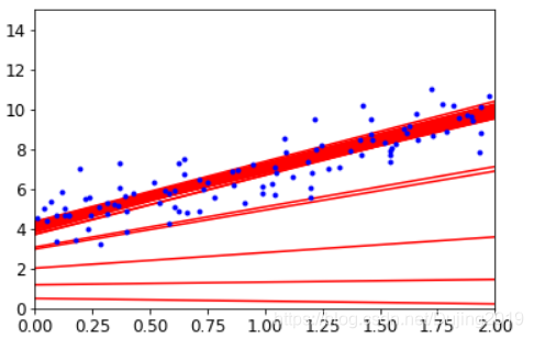
观察到当学习率比较小时，要经过很多步才能达到最终的位置，当学习率比较大时，进步的会比较快，当学习率太大的时候，学习跑偏了，没有达到饱和状态，越学习效果越差，所以学习率宁可选择小也不要选择大，至于为什么都是迭代1000次，每个图的线不一样多，是因为有的线重叠了，最终的结果值趋于稳定。

4.6 多项式回归

m = 100
X = 6*np.random.rand(m,1) - 3
y = 0.5*X**2+X+np.random.randn(m,1)

plt.plot(X,y,'b.')
plt.xlabel('X_1')
plt.ylabel('y')
plt.axis([-3,3,-5,10])
plt.show()

from sklearn.preprocessing import PolynomialFeatures
poly_features = PolynomialFeatures(degree = 2,include_bias = False)  #实例化
X_poly = poly_features.fit_transform(X)  #把数据的平方返回来
X[0]

array([2.82919615])

X_poly[0]    #第一个是x，第二个是x的平方

array([2.82919615, 8.00435083])

2.82919615 ** 2

8.004350855174822

from sklearn.linear_model import LinearRegression
lin_reg = LinearRegression()
lin_reg.fit(X_poly,y)
print (lin_reg.coef_)
print (lin_reg.intercept_)

[[1.10879671 0.53435287]]
[-0.03765461]

当前函数y=1.1x+0.53 $x^{2}$ -0.037，可以看到用PolynomialFeatures确实可以得到回归方程。

4.7 模型复杂度

#测试
X_new = np.linspace(-3,3,100).reshape(100,1)#从-3到+3按等距选出100个数
X_new_poly = poly_features.transform(X_new)  #按照相同的规则对测试数据进行转换
y_new = lin_reg.predict(X_new_poly)#用线性回归预测值
plt.plot(X,y,'b.')
plt.plot(X_new,y_new,'r--',label='prediction')   #预测结果
plt.axis([-3,3,-5,10])  #设置轴取值范围
plt.legend()
plt.show()

做对比实验，观察不同degree值得到的结果

from sklearn.pipeline import Pipeline
from sklearn.preprocessing import StandardScaler
plt.figure(figsize=(12,6))
for style,width,degree in (('g-',1,100),('b--',1,2),('r-+',1,1)):
    poly_features = PolynomialFeatures(degree = degree,include_bias = False)
    std = StandardScaler()  #标准化操作
    lin_reg = LinearRegression()  #线性回归
    polynomial_reg = Pipeline([('poly_features',poly_features),
             ('StandardScaler',std),
             ('lin_reg',lin_reg)])  #流水线1.传入poly_features 2.实例化对象3.回归操作
    polynomial_reg.fit(X,y)
    y_new_2 = polynomial_reg.predict(X_new)  #预测
    plt.plot(X_new,y_new_2,style,label = 'degree   '+str(degree),linewidth = width)
plt.plot(X,y,'b.')
plt.axis([-3,3,-5,10])
plt.legend()
plt.show()

特征变换的越复杂，得到的结果过拟合风险越高，不建议做的特别复杂。绿色在训练集上表现很好，但是在测试集上会表现很差，训练过了。

4.8 数据样本数量对结果的影响

from sklearn.metrics import mean_squared_error  #均方误差
from sklearn.model_selection import train_test_split  #对数据集进行切分操作

def plot_learning_curves(model,X,y):
    X_train, X_val, y_train, y_val = train_test_split(X,y,test_size = 0.2,random_state=100)#训练集80% 测试集20%
    train_errors,val_errors = [],[]
    for m in range(1,len(X_train)):
        model.fit(X_train[:m],y_train[:m])
        y_train_predict = model.predict(X_train[:m])
        y_val_predict = model.predict(X_val)
        train_errors.append(mean_squared_error(y_train[:m],y_train_predict[:m]))
        val_errors.append(mean_squared_error(y_val,y_val_predict))
    plt.plot(np.sqrt(train_errors),'r-+',linewidth = 2,label = 'train_error')
    plt.plot(np.sqrt(val_errors),'b-',linewidth = 3,label = 'val_error')
    plt.xlabel('Trainsing set size')
    plt.ylabel('RMSE')
    plt.legend()

lin_reg = LinearRegression()
plot_learning_curves(lin_reg,X,y)
plt.axis([0,80,0,3.3])
plt.show()

数据量越少，训练集的效果会越好，但是实际测试效果很一般，过拟合风险越大。随着数据量越来越大，过拟合风险越来越小，实际做模型的时候需要参考测试集和验证集的效果。

4.9 多项式回归的过拟合风险

polynomial_reg = Pipeline([('poly_features',PolynomialFeatures(degree = 25,include_bias = False)),
             ('lin_reg',LinearRegression())])
plot_learning_curves(polynomial_reg,X,y)
plt.axis([0,80,0,5])
plt.show()

多项式越复杂越过拟合。

4.10 正则化避免过拟合

对权重参数进行惩罚，让权重参数尽可能平滑一些，有两种不同的方法来进行正则化惩罚:

岭回归：
$J(\theta)=MSE(\theta)+\alpha\frac{1}{2}\sum_{i=1}^{n}\theta _{i}^{2}$

from sklearn.linear_model import Ridge
np.random.seed(42)
m = 20   #数据样本个数
X = 3*np.random.rand(m,1)
y = 0.5 * X +np.random.randn(m,1)/1.5 +1  
X_new = np.linspace(0,3,100).reshape(100,1)  #测试数据，从0到3选100个点

def plot_model(model_calss,polynomial,alphas,**model_kargs):
    for alpha,style in zip(alphas,('b-','g--','r:')):
        model = model_calss(alpha,**model_kargs)
        if polynomial:
            model = Pipeline([('poly_features',PolynomialFeatures(degree =10,include_bias = False)),
             ('StandardScaler',StandardScaler()),
             ('lin_reg',model)])
        model.fit(X,y)
        y_new_regul = model.predict(X_new)
        lw = 2 if alpha > 0 else 1
        plt.plot(X_new,y_new_regul,style,linewidth = lw,label = 'alpha = {}'.format(alpha))
    plt.plot(X,y,'b.',linewidth =3)
    plt.legend()

plt.figure(figsize=(14,6))
plt.subplot(121)
plot_model(Ridge,polynomial=False,alphas = (0,10,100))
plt.subplot(122)
plot_model(Ridge,polynomial=True,alphas = (0,10**-5,1))
plt.show()

lasso:

$J(\theta)=MSE(\theta)+\alpha\sum_{i=1}^{n}|\theta _{i}|$

from sklearn.linear_model import Lasso

plt.figure(figsize=(14,6))
plt.subplot(121)
plot_model(Lasso,polynomial=False,alphas = (0,0.1,1))
plt.subplot(122)
plot_model(Lasso,polynomial=True,alphas = (0,10**-1,1))
plt.show()

惩罚力度越大，alpha值越大的时候，得到的决策方程越平稳。越平稳的结果，在实际测试的时候才能发挥它的作用。

Dujing2019

发布了39 篇原创文章 · 获赞 51 · 访问量 1万+

私信关注