深度学习part1：神经网络的构建与理解

神经网络的构建与理解

一.神经网络基本框架复现

#必须放开头，否则报错。作用：把python新版本中print_function函数的特性导入到当前版本
from __future__ import print_function
import tensorflow.compat.v1 as tf#将v2版本转化成v1版本使用
tf.disable_v2_behavior()
import numpy as np
import matplotlib.pyplot as plt

#Construct a function that adds a neural layer

#inputs指输入，in_size指输入层维度，out_size指输出层维度,activation_function()指激励函数，默认None
def add_layer(inputs,in_size,out_size,activation_function=None):
    Weights=tf.Variable(tf.random.normal([in_size,out_size]))#权重
    biases=tf.Variable(tf.zeros([1,out_size])+0.1)#偏置，因为一般偏置不为0，于是人为加上0.1
    Wx_plus_b=tf.matmul(inputs,Weights)+biases#tf.matmul矩阵相乘
    if activation_function is None:
        outputs = Wx_plus_b
    else:
        outputs = activation_function(Wx_plus_b)
    return outputs

#Make up some real data

#随机x_data,这里一定要定义dtype,[:,np.newaxis]指降低一个维度
x_data = np.linspace(-1,1,300,dtype=np.float32)[:,np.newaxis]
#概率密度函数np.random.normal(loc,scale,size),loc指分布中心，scale指标准差(越小拟合的越好)，size指类型(默认size=None)
noise = np.random.normal(0,0.05,x_data.shape).astype(np.float32)
#real y_data
y_data = np.square(x_data) - 0.5 + noise

#defind placeholder for inputs to network

#此函数可以理解为形参，用于定义过程，在执行的时候再赋具体的值
xs = tf.placeholder(tf.float32,[None,1])#一定要定义tf.float32,系统不默认
ys = tf.placeholder(tf.float32,[None,1])

#add hidden layer

#这里的激励函数为relu函数，指输入层一个神经元，输出层十个神经元
l1 = add_layer(xs,1,10,activation_function = tf.nn.relu)

#add outputs layer

#这里激励函数为None
prediction = add_layer(l1,10,1,activation_function = None)

#the error between real data and prediction

#定义loss，指损失函数总和的平均值，注意这里必须得加上一个reduction_indices=[]。(会说明)
loss = tf.reduce_mean(tf.reduce_sum(tf.square(ys - prediction),reduction_indices=[1]))
#这里用GradientDescentOptimizer做为优化器,就是梯度下降法
train_step = tf.train.GradientDescentOptimizer(0.1).minimize(loss)

#Activate
sess = tf.Session()#非常重要

#定义全局初始化(两种表示方法:global_variables_initializer,initialize_all_variables)
#建议用global_variables_initializer新版本
init = tf.global_variables_initializer()

sess.run(init)
for i in range(1000):
	#train,这里的feed_dict是一个字典，用于导入数据x_data和y_data
    sess.run(train_step,feed_dict = {xs : x_data, ys : y_data})
    #每50步打印一次
    if i % 50 == 0:
        print(sess.run(loss,feed_dict = {xs : x_data, ys : y_data}))

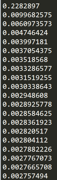
显示结果

显然loss不断趋近于0

部分代码解释

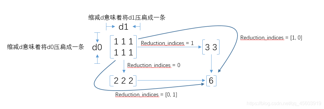
当我们计算loss时必须加上reduction_indices=[1],这是一个函数的处理维度。如果没有这个函数默认值为0，则train_step将会被降维成一个数(0维)

reduction_indices工作原理图

优化器的种类（图片）

新手可以使用GradientDescentOptimizer
进阶一点可以使用MomenttumOptimizer或AdamOptimizer

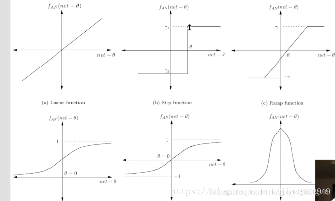
激励函数的种类（图片）

二.结果可视化

#Visualization of results
fig = plt.figure()#建立一个背景
ax = fig.add_subplot(1,1,1)#建立标注
ax.scatter(x_data , y_data)#scatter指散点
plt.ion()#全局变量时，最好注释掉。作用：使图像连续
plt.show()
for i in range(1000):
    # training
    sess.run(train_step, feed_dict={xs: x_data, ys: y_data})
    if i % 50 == 0:
        # to visualize the result and improvement
        #指没有图像就跳过(简单理解：先抹去线，再出现下一次线)
        try:
            ax.lines.remove(lines[0])
        except Exception:
            pass
        prediction_value = sess.run(prediction, feed_dict={xs: x_data})
        # plot the prediction
        lines = ax.plot(x_data, prediction_value, 'r-', lw=3)#红色，宽度为3
        plt.pause(0.1)#指暂停几秒，作者实验表明0.1~0.3可视化效果明显

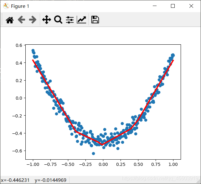
效果图(还是有误差)

Ending！