SSD: Single Shot MultiBox Detector（SSD 论文翻译）

---

英文版论文原文：https://arxiv.org/pdf/1512.02325.pdf

---

SSD: Single Shot MultiBox Detector

Wei Liu,Dragomir Anguelov ,Dumitru Erhan ,Christian Szegedy ,Scott Reed ,Cheng-Yang Fu & Alexander C. Berg

• UNC Chapel Hill
• Zoox Inc
• Google Inc
• University of Michigan, Ann-Arbor

Abstract

提出了一种利用单个深度神经网络对图像中目标进行检测的方法。我们的方法名为SSD，它将边界框的输出空间离散为一组默认框，每个特征映射位置具有不同的纵横比和比例。在预测时，网络为每个默认框中每个对象类别的存在生成评分，并对该框进行调整以更好地匹配对象形状。此外，该网络结合了来自具有不同分辨率的多个特征图的预测，以自然地处理不同大小的对象。相对于需要对象建议的方法，SSD比较简单，因为它完全消除了建议生成和随后的像素或特征重采样阶段，并将所有计算封装在一个网络中。这使得SSD易于培训，并且易于集成到需要检测组件的系统中。在PASCAL VOC、COCO和ILSVRC数据集上的实验结果证实，相对于使用附加对象建议步骤的方法，SSD具有竞争力的准确性，而且速度更快，同时为训练和推理提供了统一的框架。对于300×300输入，SSD在Nvidia Titan X上以59 FPS的速度在VOC2007测试上达到74.3％的mAP1;对于512×512输入，SSD达到76.9％的mAP，优于同类的最新Faster R-CNN模型。与其他单阶段方法相比，即使输入图像尺寸较小，SSD的精度也要好得多。代码可在以下网址获得：https：//github.com/weiliu89/caffe/tree/ssd。

We present a method for detecting objects in images using a single deep neural network. Our approach, named SSD, discretizes the output space of bounding boxes into a set of default boxes over different aspect ratios and scales per feature map location. At prediction time, the network generates scores for the presence of each object category in each default box and produces adjustments to the box to better match the object shape. Additionally, the network combines predictions from multiple feature maps with different resolutions to naturally handle objects of various sizes. SSD is simple relative to methods that require object proposals because it completely eliminates proposal generation and subsequent pixel or feature resampling stages and encapsulates all computation in a single network. This makes SSD easy to train and straightforward to integrate into systems that require a detection component. Experimental results on the PASCAL VOC, COCO, and ILSVRC datasets confirm that SSD has competitive accuracy to methods that utilize an additional object proposal step and is much faster, while providing a unified framework for both training and inference. For 300 × 300 input, SSD achieves 74.3% mAP1 on VOC2007 test at 59 FPS on a Nvidia Titan X and for 512 × 512 input, SSD achieves 76.9% mAP, outperforming a comparable state-of-the-art Faster R-CNN model. Compared to other single stage methods, SSD has much better accuracy even with a smaller input image size. Code is available at: https://github.com/weiliu89/caffe/tree/ssd .

1 Introduction

当前最新的对象检测系统是以下方法的变体：假设边界框，为每个框重新采样像素或特征，并应用高质量的分类器。自从选择性搜索工作[1]以来，该管道就一直在检测基准上占主导地位，尽管基于PASCAL VOC，COCO和ILSVRC检测的当前领先结果全部基于Faster R-CNN [2]，尽管具有更深的功能，例如[3]。虽然这些方法准确无误，但对于嵌入式系统而言，它们的计算量很大，即使使用高端硬件也是如此，对于实时应用程序来说却太慢了。这些方法的检测速度通常以每帧秒数（SPF）来衡量，甚至是最快的高精度检测器Faster R-CNN，仅以每秒7帧（FPS）的速度运行。已经有很多尝试通过攻击检测管线的每个阶段来构建更快的检测器（请参见第4节中的相关工作），但是到目前为止，速度的显着提高仅是以大大降低检测精度为代价的。

Current state-of-the-art object detection systems are variants of the following approach: hypothesize bounding boxes, resample pixels or features for each box, and apply a high-quality classifier. This pipeline has prevailed on detection benchmarks since the Selective Search work [1] through the current leading results on PASCAL VOC, COCO, and ILSVRC detection all based on Faster R-CNN[2] albeit with deeper features such as [3]. While accurate, these approaches have been too computationally intensive for embedded systems and, even with high-end hardware, too slow for real-time applications.Often detection speed for these approaches is measured in seconds per frame (SPF), and even the fastest high-accuracy detector, Faster R-CNN, operates at only 7 frames per second (FPS). There have been many attempts to build faster detectors by attacking each stage of the detection pipeline (see related work in Sec. 4), but so far, significantly increased speed comes only at the cost of significantly decreased detection accuracy.

本文提出了一种基于深度网络的目标检测器，它不需要对像素或特征进行重新采样，也不需要对边界框假设进行重新采样，并且与现有方法一样精确。这使得高精度检测的速度有了显著提高(在VOC2007测试中，59帧FPS (mAP 74.3%)，而faster R-CNN 7帧FPS (mAP 73.2%)或YOLO 45帧FPS (mAP 63.4%)。速度的根本改进来自消除边框建议和随后的像素或特征重采样阶段。我们并不是第一个这样做的人(cf[4,5])，但是通过添加一系列改进，我们能够比以前的尝试显著提高准确度。我们的改进包括：使用小型卷积滤波器来预测对象类别和边界框位置中的偏移；使用单独的预测器（滤波器）进行不同的宽高比检测；以及将这些滤波器应用于网络后期的多个特征图，以便执行多尺度检测。通过这些修改（尤其是使用多层进行不同规模的预测），我们可以使用相对较低的分辨率输入来实现高精度，从而进一步提高检测速度。尽管这些贡献似乎很小，但我们注意到，结果系统将PASCAL VOC的实时检测精度从YOLO的63.4％mAP提高到了SSD的74.3％mAP。与最近在残差网络上非常引人注目的工作相比，这在检测精度上有较大的相对提高[3]。此外，显着提高高质量检测的速度可以拓宽使用计算机视觉的设置范围。

This paper presents the first deep network based object detector that does not resample pixels or features for bounding box hypotheses and and is as accurate as approaches that do. This results in a significant improvement in speed for high-accuracy detection (59 FPS with mAP 74.3% on VOC2007 test, vs. Faster R-CNN 7 FPS with mAP 73.2% or YOLO 45 FPS with mAP 63.4%). The fundamental improvement in speed comes from eliminating bounding box proposals and the subsequent pixel or feature resampling stage. We are not the first to do this (cf [4,5]), but by adding a series of improvements, we manage to increase the accuracy significantly over previous attempts. Our improvements include using a small convolutional filter to predict object categories and offsets in bounding box locations, using separate predictors (filters) for different aspect ratio detections, and applying these filters to multiple feature maps from the later stages of a network in order to perform detection at multiple scales. With these modifications—especially using multiple layers for prediction at different scales—we can achieve high-accuracy using relatively low resolution input, further increasing detection speed. While these contributions may seem small independently, we note that the resulting system improves accuracy on real-time detection for PASCAL VOC from 63.4% mAP for YOLO to 74.3% mAP for our SSD. This is a larger relative improvement in detection accuracy than that from the recent, very high-profile work on residual networks [3]. Furthermore, significantly improving the speed of high-quality detection can broaden the range of settings where computer vision is useful.

我们将我们的贡献总结如下：

We summarize our contributions as follows:

• 我们推出了SSD，这是一种适用于多种类别的单发检测器，它比以前的最新单发检测器（YOLO）速度更快，并且精度更高，实际上与执行显式区域建议和池化(包括faster R-CNN)的较慢技术一样准确。

We introduce SSD, a single-shot detector for multiple categories that is faster than the previous state-of-the-art for single shot detectors (YOLO), and significantly more accurate, in fact as accurate as slower techniques that perform explicit region proposals and pooling (including Faster R-CNN).

• SSD的核心是使用应用于特征图的小型卷积滤波器，为一组固定的默认边界框预测类别得分和框偏移。

The core of SSD is predicting category scores and box offsets for a fixed set of default bounding boxes using small convolutional filters applied to feature maps.

• 为了获得较高的检测精度，我们从不同比例的特征图生成不同比例的预测，并按宽高比将显示明确分开。

To achieve high detection accuracy we produce predictions of different scales from feature maps of different scales, and explicitly separate predictions by aspect ratio.

• 这些设计功能即使在低分辨率输入图像上也可以实现简单的端到端训练和高精度，从而进一步提高了速度与精度之间的权衡。

These design features lead to simple end-to-end training and high accuracy, even on low resolution input images, further improving the speed vs accuracy trade-off.

• 实验包括对通过PASCAL VOC，COCO和ILSVRC评估的具有可变输入大小的模型进行时序和精度分析，并将其与一系列最新技术进行了比较。

Experiments include timing and accuracy analysis on models with varying input size evaluated on PASCAL VOC, COCO, and ILSVRC and are compared to a range of recent state-of-the-art approaches.

2. 单发检测器（SSD）

2 The Single Shot Detector (SSD)

本节介绍我们提出的用于检测的SSD框架(第2.1节)和相关的训练方法(第2.2节)。然后，第3节给出了特定于数据集的模型细节和实验结果。

This section describes our proposed SSD framework for detection (Sec. 2.1) and the associated training methodology (Sec. 2.2). Afterwards, Sec. 3 presents dataset-specific model details and experimental results.

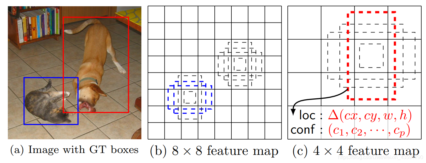
图1：SSD框架。 （a）在训练过程中，SSD仅需要每个对象的输入图像和地面真相框。 以卷积方式，我们在几张具有不同比例（例如（b）和（c）中的8×8和4×4）的特征图中，评估了每个位置上一小组不同纵横比的默认框（例如4个）。 对于每个默认框，我们预测所有对象类别（ $(c_1, c_2, ...,c_p)$ ）的形状偏移量和置信度。 在训练时，我们首先将这些默认框与地面真相框进行匹配。 例如，我们将两个默认框与猫匹配，将一个默认框与狗匹配，这两个默认框被视为正，而其余框被视为负。 模型损失是定位损失（例如，平滑L1 [6]）和置信度损失（例如，Softmax）之间的加权总和。

Fig. 1: SSD framework. (a) SSD only needs an input image and ground truth boxes for each object during training. In a convolutional fashion, we evaluate a small set (e.g. 4) of default boxes of different aspect ratios at each location in several feature maps with different scales (e.g. 8 × 8 and 4 × 4 in (b) and ©). For each default box, we predict both the shape offsets and the confidences for all object categories ( $(c_1, c_2, ...,c_p)$). At training time, we first match these default boxes to the ground truth boxes. For example, we have matched two default boxes with the cat and one with the dog, which are treated as positives and the rest as negatives. The model loss is a weighted sum between localization loss (e.g. Smooth L1 [6]) and confidence loss (e.g. Softmax).

2.1 Model

SSD方法基于前馈卷积网络，该网络产生固定大小的边界框集合，并为这些框中存在的对象类实例打分，然后进行非最大抑制步骤以产生最终检测结果。 早期的网络层基于用于高质量图像分类的标准体系结构（在任何分类层之前均被截断），我们将其称为基础网络2。 然后，我们将辅助结构添加到网络，以产生具有以下关键特征的检测结果：

The SSD approach is based on a feed-forward convolutional network that produces a fixed-size collection of bounding boxes and scores for the presence of object class instances in those boxes, followed by a non-maximum suppression step to produce the final detections. The early network layers are based on a standard architecture used for high quality image classification (truncated before any classification layers), which we will call the base network2. We then add auxiliary structure to the network to produce detections with the following key features:

用于检测的 多尺度特征图 我们将卷积特征层添加到截断的基础网络的末尾。 这些层的大小逐渐减小，并可以预测多个尺度的检测。 对于每个特征层，用于预测检测的卷积模型是不同的（参见在单个比例尺特征图上运行的Overfeat [4]和YOLO [5]）。

Multi-scale feature maps for detection We add convolutional feature layers to the end of the truncated base network. These layers decrease in size progressively and allow predictions of detections at multiple scales. The convolutional model for predicting detections is different for each feature layer (cf Overfeat[4] and YOLO[5] that operate on a single scale feature map).

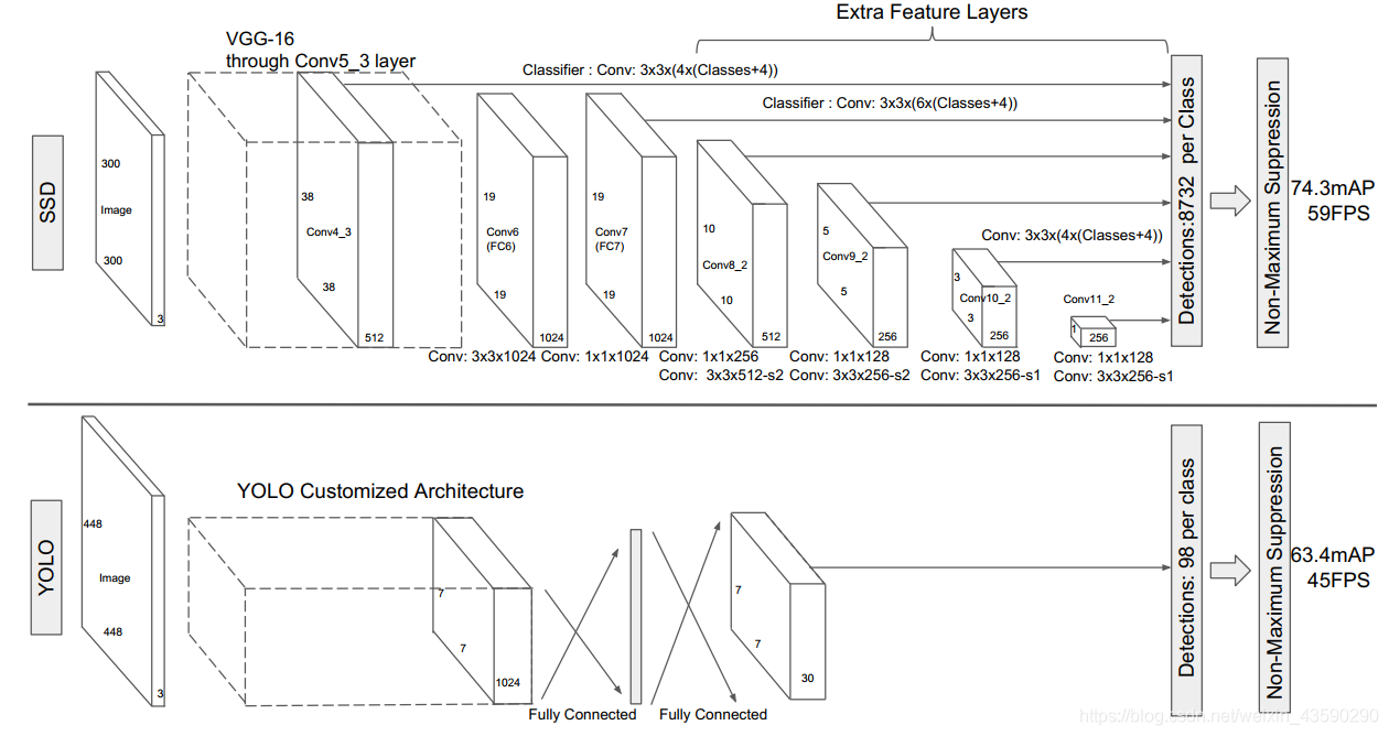
图2：SSD和YOLO两种单发检测模型之间的比较[5]。 我们的SSD模型在基础网络的末尾添加了几个功能层，这些功能层可预测与不同比例和纵横比的默认框的偏移量及其关联的置信度。 在VOC2007测试中，具有300×300输入尺寸的SSD在精度上明显优于其448×448 YOLO同类产品，同时还提高了速度。

Fig. 2: A comparison between two single shot detection models: SSD and YOLO [5]. Our SSD model adds several feature layers to the end of a base network, which predict the offsets to default boxes of different scales and aspect ratios and their associated confidences. SSD with a 300 × 300 input size significantly outperforms its 448 × 448 YOLO counterpart in accuracy on VOC2007 test while also improving the speed.

用于检测的卷积预测变量每个添加的特征层（或可选地，来自基础网络的现有特征层）都可以使用一组卷积滤波器生成一组固定的检测预测。 这些在图2的SSD网络体系结构的顶部表示。对于具有p个通道的 $m×n$n大小的特征层，预测电位检测参数的基本元素是 $3×3×p$ 小内核 会产生类别得分或相对于默认框坐标的形状偏移。 在应用内核的 $m×n$ 个位置中的每个位置，它都会产生一个输出值。 边界框偏移输出值是相对于相对于每个要素地图位置的默认框位置进行测量的（参见YOLO [5]的体系结构，该过程使用中间完全连接层而不是卷积滤波器进行此步骤）。

Convolutional predictors for detection Each added feature layer (or optionally an existing feature layer from the base network) can produce a fixed set of detection predictions using a set of convolutional filters. These are indicated on top of the SSD network architecture in Fig. 2. For a feature layer of size $m × n$ with p channels, the basic element for predicting parameters of a potential detection is a $3 × 3 × p$ small kernel that produces either a score for a category, or a shape offset relative to the default box coordinates. At each of the $m × n$ locations where the kernel is applied, it produces an output value. The bounding box offset output values are measured relative to a default box position relative to each feature map location (cf the architecture of YOLO[5] that uses an intermediate fully connected layer instead of a convolutional filter for this step).

默认框和纵横比 我们将一组默认边界框与每个要素图单元相关联，以用于网络顶部的多个要素图。默认框以卷积方式平铺要素图，因此每个框相对于其对应单元格的位置是固定的。在每个要素贴图单元中，我们预测相对于单元中默认框形状的偏移量，以及每个类得分，这些得分指示每个类框中都存在类实例。具体来说，对于给定位置k中的每个盒子，我们计算c类得分和相对于原始默认盒子形状的4个偏移量。这将导致在特征图中每个位置周围应用 $(c + 4)k$ 个滤镜，从而为 $m × n$ 特征图产生 $(c + 4)kmn$ 个输出。有关默认框的说明，请参阅图1。我们的默认框与Faster R-CNN [2]中使用的锚框相似，但是我们将它们应用于多个不同分辨率的特征图。在几个要素图中允许使用不同的默认盒子形状，可以使我们有效地离散可能的输出盒子形状的空间。

Default boxes and aspect ratios We associate a set of default bounding boxes with each feature map cell, for multiple feature maps at the top of the network. The default boxes tile the feature map in a convolutional manner, so that the position of each box relative to its corresponding cell is fixed. At each feature map cell, we predict the offsets relative to the default box shapes in the cell, as well as the per-class scores that indicate the presence of a class instance in each of those boxes. Specifically, for each box out of k at a given location, we compute c class scores and the 4 offsets relative to the original default box shape. This results in a total of $(c + 4)k$ filters that are applied around each location in the feature map, yielding $(c + 4)kmn$ outputs for a $m × n$ feature map. For an illustration of default boxes, please refer to Fig. 1. Our default boxes are similar to the anchor boxes used in Faster R-CNN [2], however we apply them to several feature maps of different resolutions. Allowing different default box shapes in several feature maps let us efficiently discretize the space of possible output box shapes.

2.2 Training

训练SSD和训练使用区域建议的典型探测器之间的主要区别在于，需要将地面真实信息分配给探测器输出的固定集合中的特定输出。 在YOLO [5]中的训练以及Faster R-CNN [2]和MultiBox [7]的区域提议阶段，也都需要此版本。 确定此分配后，将损耗函数和反向传播端到端应用。 训练还涉及选择一组默认的检测框和标尺进行检测，以及严格的否定挖掘和数据增强策略。

The key difference between training SSD and training a typical detector that uses region proposals, is that ground truth information needs to be assigned to specific outputs in the fixed set of detector outputs. Some version of this is also required for training in YOLO[5] and for the region proposal stage of Faster R-CNN[2] and MultiBox[7]. Once this assignment is determined, the loss function and back propagation are applied end-to-end. Training also involves choosing the set of default boxes and scales for detection as well as the hard negative mining and data augmentation strategies.

匹配策略 在训练期间，我们需要确定哪些默认框对应于地面真相检测，并相应地训练网络。 对于每个地面真相框，我们从默认框中进行选择，这些默认框随位置，宽高比和比例而变化。 我们首先将每个地面真值框与具有最佳提花卡重叠的默认框进行匹配（如MultiBox [7]）。 与MultiBox不同，我们随后将默认框与jaccard重叠高于阈值（0.5）的所有地面实况进行匹配。 这简化了学习问题，使网络能够为多个重叠的默认框预测高分，而不是要求它仅选择重叠最大的框。

Matching strategy During training we need to determine which default boxes correspond to a ground truth detection and train the network accordingly. For each ground truth box we are selecting from default boxes that vary over location, aspect ratio, and scale. We begin by matching each ground truth box to the default box with the best jaccard overlap (as in MultiBox [7]). Unlike MultiBox, we then match default boxes to any ground truth with jaccard overlap higher than a threshold (0.5). This simplifies the learning problem, allowing the network to predict high scores for multiple overlapping default boxes rather than requiring it to pick only the one with maximum overlap.

训练目标SSD训练目标是从MultiBox目标[7,8]派生而来的，但可以扩展为处理多个对象类别。 令 $x^p_{ij} = {1,0}$ 是一个指标，用于将第j个默认框与类别p的第j个地面真实框进行匹配。 在上面的匹配策略中，我们可以有 $\sum_ix^p_{ij} \ge 1$ 。 总体目标损失函数是定位损失（loc）和置信度损失（conf）的加权和：

Training objective The SSD training objective is derived from the MultiBox objective [7,8] but is extended to handle multiple object categories. Let $x^p_{ij} = {1,0}$ be an indicator for matching the j-th default box to the j-th ground truth box of category p. In the matching strategy above, we can have $\sum_ix^p_{ij} \ge 1$. The overall objective loss function is a weighted sum of the localization loss (loc) and the confidence loss (conf):

$\tag{1} L(x,c,l,g)=\frac{1}{N}(L_{conf}(x,c)+\alpha L_{loc}(x,l,g))$

其中N是匹配的默认框的数量。 如果 $N = 0$ ，则将损失设为0。定位损失是预测框 $(l)$ 和地面真实框 $(g)$ 参数之间的平滑L1损失[6]。 与Faster R-CNN [2]类似，我们回归到默认边界框 $(d)$ 的中心 $(cx,cy)$ 及其宽度 $(w)$ 和高度 $(h)$ 的偏移量。

where N is the number of matched default boxes. If $N = 0$, wet set the loss to 0. The localization loss is a Smooth L1 loss [6] between the predicted box $(l)$ and the ground truth box $(g)$ parameters. Similar to Faster R-CNN [2], we regress to offsets for the center $(cx,cy)$ of the default bounding box $(d)$ and for its width $(w)$ and height $(h)$.

$L_{loc}(x,l,g)=\displaystyle\sum_{i\in Pos}^N \displaystyle\sum_{m\in {cx,cy,w,h}}x^k_{ij}smooth_{L1}(l_i^m-\hat{g}^m_j)$

$\tag{2} \hat{g}^{cx}_j =(g^{cx}_j-d^{cx}_i)/d^w_i \space \space\space\space\space\space\space \hat{g}^{cy}_j=(g^{cy}_j-d^{cy}_i)/d_i^h$

$\hat{g}^w_j=log(\frac{g^w_j}{d^w_i}) \space \space\space\space\space\space\space \hat{g}^h_j=log(\frac{g^h_j}{d_i^h})$

置信度损失是多个类别置信度（c）上的softmax损失。

The confidence loss is the softmax loss over multiple classes confidences ©.

$\tag{3} L_{conf}(x,c)=-\displaystyle\sum_{i\in Pos}^N x^p_{ij}log(\hat{c}^p_i)-\displaystyle\sum_{i\in Neg}log()\hat{c^0_i} \space\space where \space\space \hat{c}^p_i=\frac{exp(c^p_i)}{\sum_p exp(c^p_i)}$

权项 $α$ 通过交叉验证设置为1。

and the weight term $α$ is set to 1 by cross validation.