目录
GAN
论文链接 Generative Adversarial Nets
问题:数据x分布为 \(P_{data}(x)\),有样本{\({x_1,x_2,...,x_m}\)}。现在我们有生成器 \(G\) ,希望生成器 \(G\)生成这些样本的概率最大。似然是
\(L = \sum_{i=1}^{m}P_G{(x_i;\theta)}\), \(\theta\)为G的参数。
极大似然估计:\(\theta^* = arg\ \underset{\theta}{max}\prod_{i=1}^{m}P_G({x_i;\theta})\)

第四行假设样本独立同分布,\(m\)越大越好。
第五行加了一个与\(\theta\)无关的项,相当于\(D(p||q) = H(p,q) - H(p)\),其实没必要。
这样当\(P_{data}(x)=P_G (x)\) 时,似然最大。
接下来GAN登场,

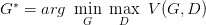
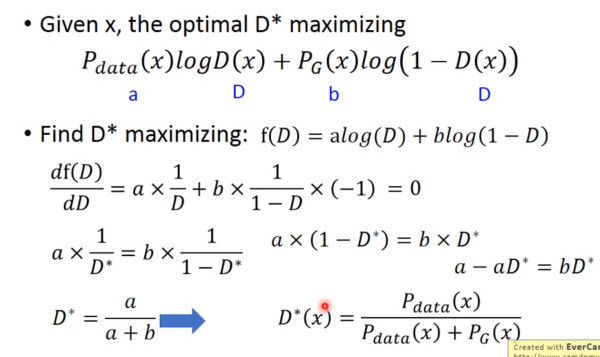
固定\(G\),求得最好的\(D\)
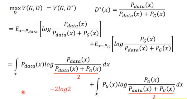
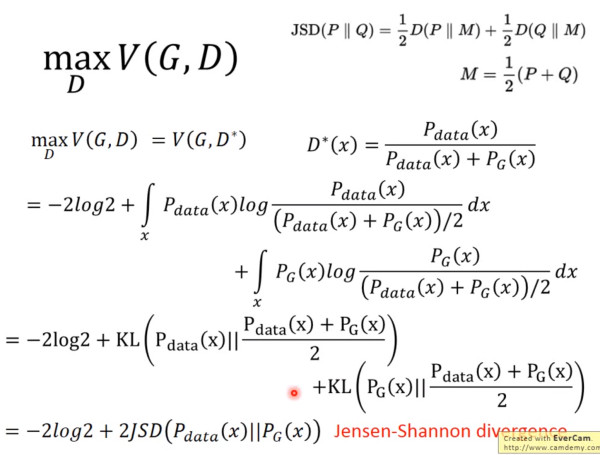
所以当 \(P_{data}=P_{G}\)时,\(G\)最优,原来的极大似然估计,转变成了GAN
上面都是理论,明白就行。
具体算法:

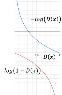
但是 \(log(1-D(x))\)在\(D(x)=0\)处太平滑,\(D(x)\)接近1时反而太大,接近刚开始\(G\)很弱,\(D(G(z))\)很小,用
\(-log(D(x))\)代替正好合适。
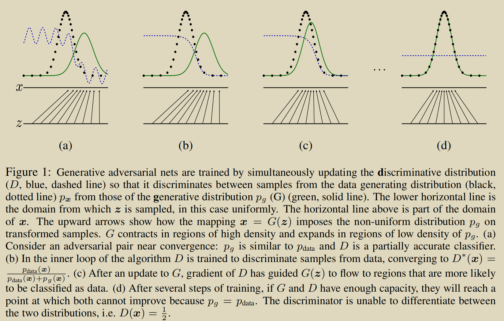
很直观的描述训练过程
#Pytorch 实现loss
adversarial_loss=torch.nn.BCELoss()
g_loss = adversarial_loss(discriminator(gen_imgs), valid) # valid全1序列,fake全0序列
real_loss = adversarial_loss(discriminator(real_imgs), valid)
fake_loss = adversarial_loss(discriminator(gen_imgs.detach()), fake) #detach()在这里不管
d_loss = (real_loss + fake_loss) / 2
BCELoss:
\[\ell(x, y) = mean(L) = mean(\{l_1,\dots,l_N\}^\top), \quad l_n = - w_n \left[ y_n \cdot \log x_n + (1 - y_n) \cdot \log (1 - x_n) \right]\]

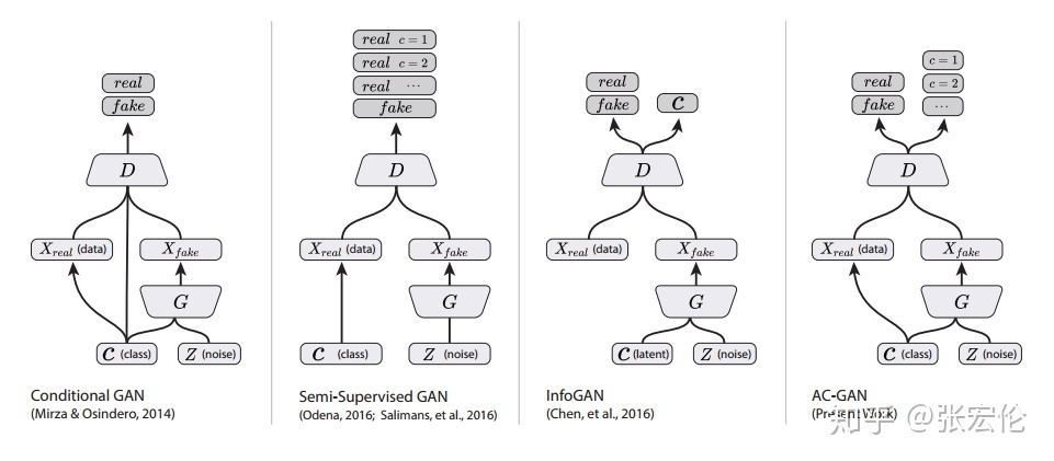
ACGAN
能够控制生成类别,
G第一层:self.label_emb = nn.Embedding(opt.n_classes, opt.latent_dim)
使用embedding的方法。
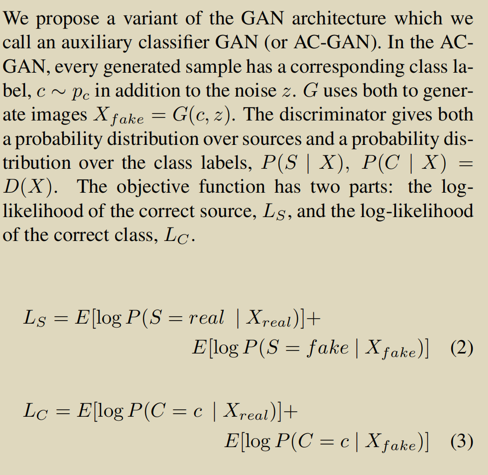
\(D\) is trained to maximize \(L_S + L_C\) while \(G\) is trained to maximize \(L_C − L_S\). AC-GANs learn a representation for \(z\) that is independent of class label
validity, pred_label = discriminator(gen_imgs)
g_loss = 0.5 * (adversarial_loss(validity, valid) + auxiliary_loss(pred_label, gen_labels))
real_pred, real_aux = discriminator(real_imgs)
d_real_loss=(adversarial_loss(real_pred, valid) + auxiliary_loss(real_aux, labels))/2
# Loss for fake images
fake_pred, fake_aux = discriminator(gen_imgs.detach())
d_fake_loss=(adversarial_loss(fake_pred, fake) + auxiliary_loss(fake_aux, gen_labels))/2
# Total discriminator loss
d_loss = (d_real_loss + d_fake_loss) / 2CrossEntropyLoss:
\[ \text{loss}(x, class) = -\log\left(\frac{\exp(x[class])}{\sum_j \exp(x[j])}\right) = -x[class] + \log\left(\sum_j \exp(x[j])\right)\]
AAE

encoded_imgs = encoder(real_imgs)
decoded_imgs = decoder(encoded_imgs)

# Loss measures generator's ability to fool the discriminator
g_loss = 0.001 * adversarial_loss(discriminator(encoded_imgs), valid) + 0.999 * pixelwise_loss(decoded_imgs, real_imgs)
z = Variable(Tensor(np.random.normal(0, 1, (imgs.shape[0], opt.latent_dim))))
# Measure discriminator's ability to classify real from generated samples
real_loss = adversarial_loss(discriminator(z), valid)
fake_loss = adversarial_loss(discriminator(encoded_imgs.detach()), fake)
d_loss = 0.5 * (real_loss + fake_loss)
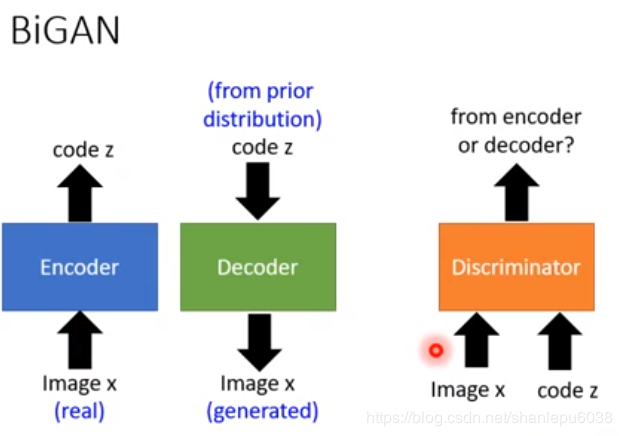
BiGAN
BGAN
def boundary_seeking_loss(y_pred, y_true):
    """
    Boundary seeking loss.
    Reference: https://wiseodd.github.io/techblog/2017/03/07/boundary-seeking-gan/
    """
    return 0.5 * torch.mean((torch.log(y_pred) - torch.log(1 - y_pred)) ** 2)
g_loss = boundary_seeking_loss(discriminator(gen_imgs), valid)
适用于离散数据
BEGAN
BEGAN: Boundary Equilibrium Generative Adversarial Networks
两个贡献:
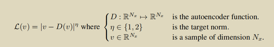
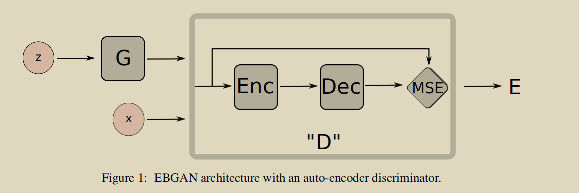
1.使用autoencoder作为D
\(L : R^{N_x} \to R^+\) the loss for training a pixel-wise autoencoder as:
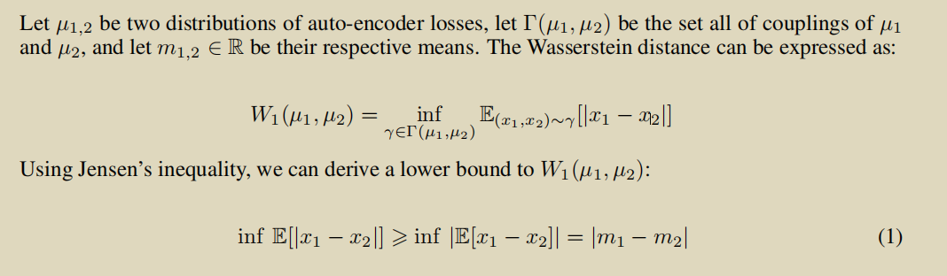
使用Wasserstein loss来衡量real_loss和fake_loss分布之间的差距

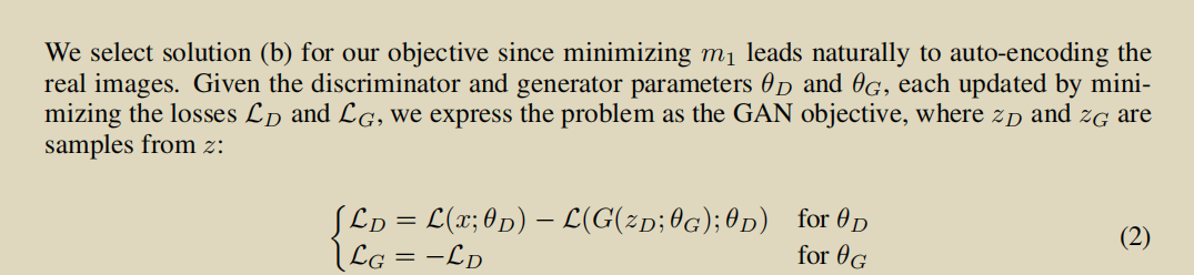
选择上面的b因为,一个好的D是对real友好的。
g_loss = torch.mean(torch.abs(discriminator(gen_imgs) - gen_imgs))2.使用了 Equilibrium
收敛的时候我们希望\(E(L(x))=E(L(G(z)))\),但是我们可以relax一下这个条件
\(\gamma = \frac{E(L(G(z))}{E(L(x))}\) ,\(\gamma\in[0,1]\)
(因为G不强,所以autoencoder可以轻松模拟G生成的图像,\(L(G(z))\)很小)
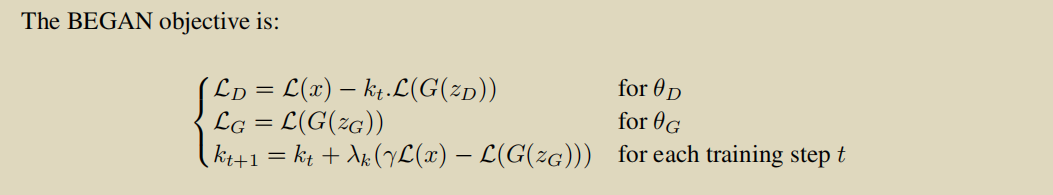
用了Proportional Control Theory使得\(E [L(G(z))] = γE [L(x)]\)
\(M_{global} = L(x) + |γL(x) − L(G(zG))|\)用来衡量是否收敛
 d_real = discriminator(real_imgs)
 d_fake = discriminator(gen_imgs.detach())

 d_loss_real = torch.mean(torch.abs(d_real - real_imgs))
 d_loss_fake = torch.mean(torch.abs(d_fake - gen_imgs.detach()))
 d_loss = d_loss_real - k * d_loss_fake
 diff = torch.mean(gamma * d_loss_real - d_loss_fake)

 # Update weight term for fake samples
 k = k + lambda_k * diff.item()
 k = min(max(k, 0), 1)  # Constraint to interval [0, 1]
 # Update convergence metric
 M = (d_loss_real + torch.abs(diff)).item()
BicycleGAN
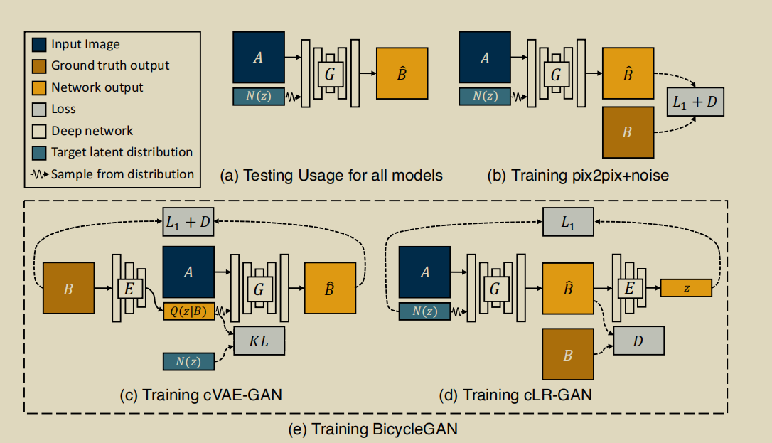
训练完成后,使用G,给定A,微调z就可以生成不同的图像。
没什么重点,训练的时候注意一下更新参数的顺序就行了
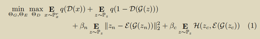
ClusterGAN
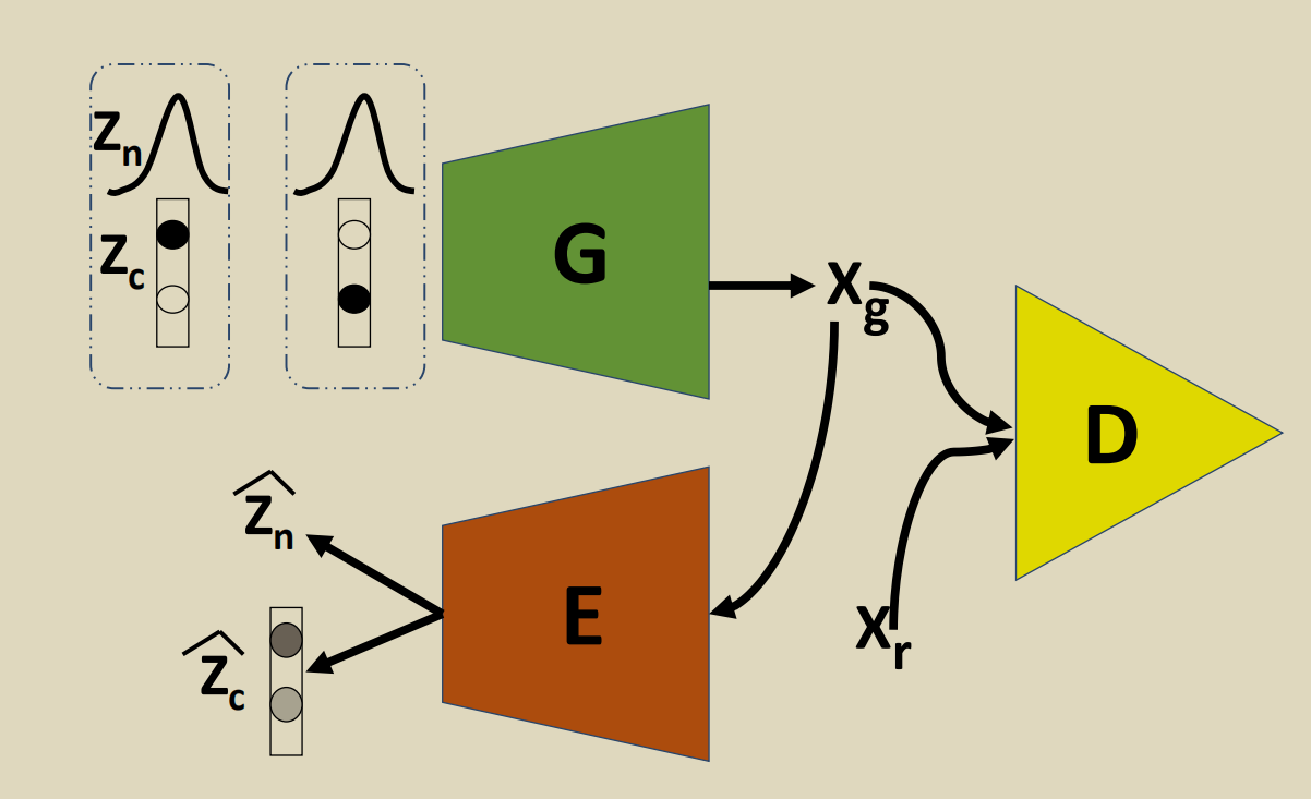
利用离散连续混合采样,平衡聚类和插值。
损失函数\(q(x)\) 是可以使\(q(x)=log(x)\)或者是\(q(x)=x\)(WGAN)
CGAN

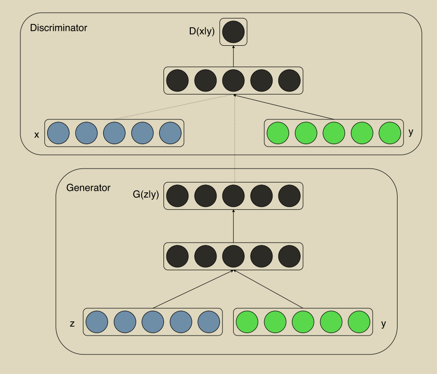
D需要y的输入,因为D需要知道这个条件,否则G可以生成随便的高质量的图片
$\underset{G}{Min} \underset{D}{Min}V(D, G) = E_{x∼ p_{data}(x)}[log D(x|y)] + E_{z∼p_z(z)}[log(1 − D(G(z|y)))]. $
G loss
        z = Variable(FloatTensor(np.random.normal(0, 1, (batch_size, opt.latent_dim))))
        gen_labels = Variable(LongTensor(np.random.randint(0, opt.n_classes, batch_size)))

        # Generate a batch of images
        gen_imgs = generator(z, gen_labels)

        # Loss measures generator's ability to fool the discriminator
        validity = discriminator(gen_imgs, gen_labels)
        g_loss = adversarial_loss(validity, valid)
D loss
        validity_real = discriminator(real_imgs, labels)
        d_real_loss = adversarial_loss(validity_real, valid)

        # Loss for fake images
        validity_fake = discriminator(gen_imgs.detach(), gen_labels)
        d_fake_loss = adversarial_loss(validity_fake, fake)

        # Total discriminator loss
        d_loss = (d_real_loss + d_fake_loss) / 2
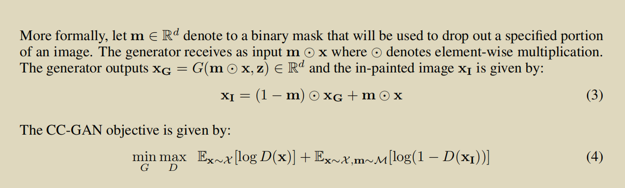
CCGAN
SEMI-SUPERVISED LEARNING WITH CONTEXT-CONDITIONAL GENERATIVE ADVERSARIAL NETWORKS
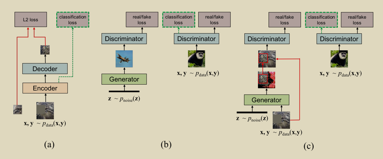
第二个版本,更加重视对fake的判断
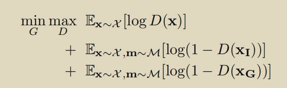
第三个版本
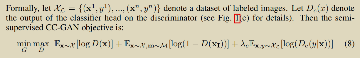
半监督学习的思想:
将D看做是一个分类器,(x,y)带标签的数据正常分类,假的生成的fake看作是第k+1类,真的image无标签,判断其不是第k+1类的概率
Context Encoders
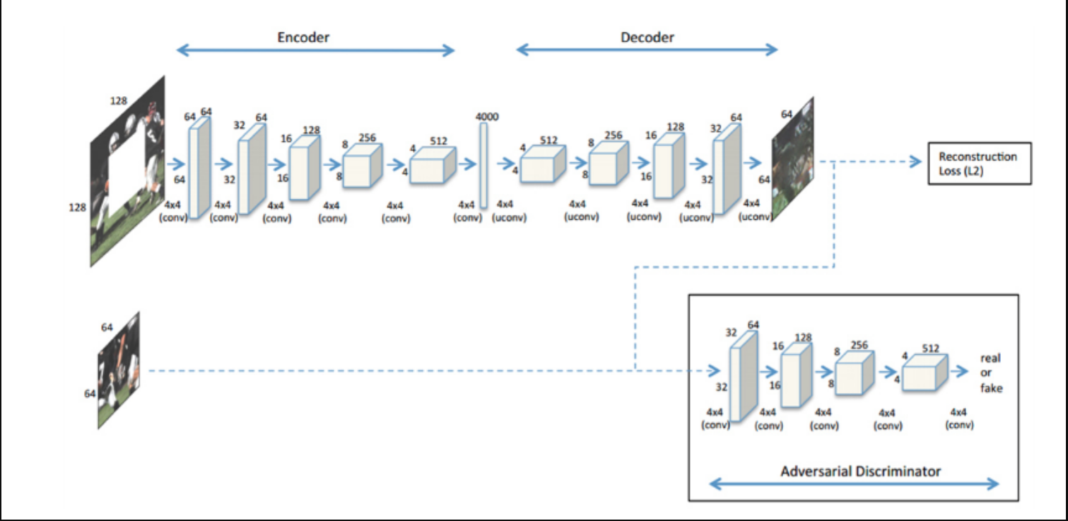

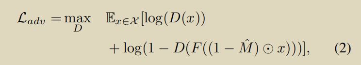
跟上面一篇基本一样,没什么可说的
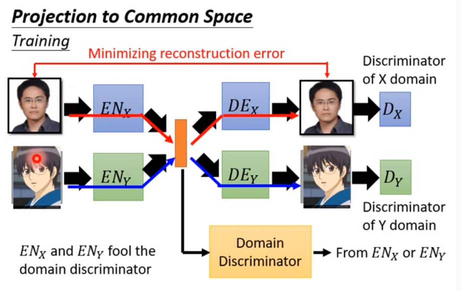
CoGAN

通过参数共享,通过两个边缘分布,就可以学习到两个分布的联合分布
另一种形式,也可以用下面的形式,或者,加参数共享,cycle,等保证中间的latent-space分布一致
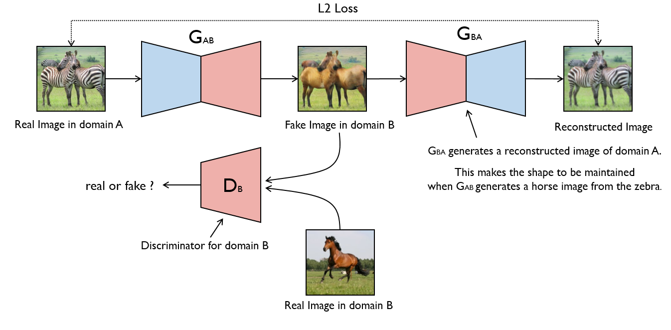
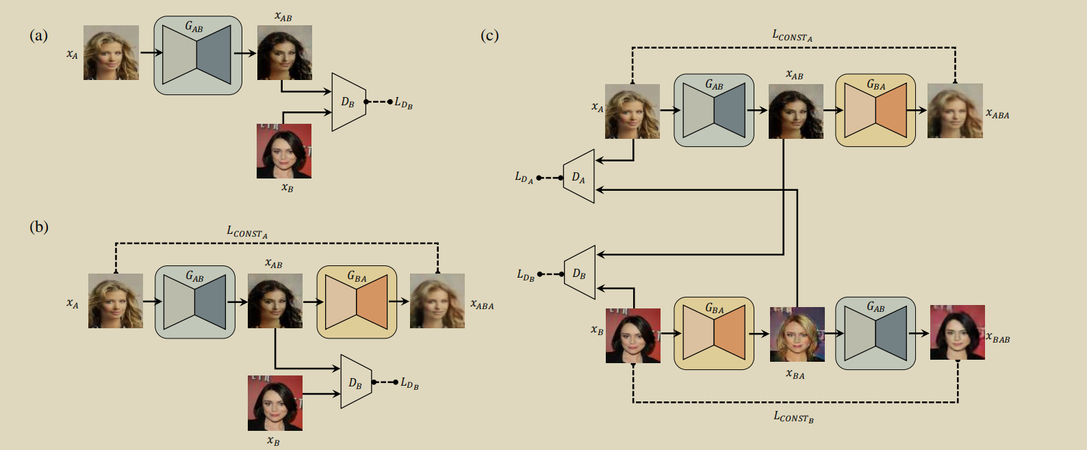
CycleGAN
 # Set model input
        real_A = Variable(batch["A"].type(Tensor))
        real_B = Variable(batch["B"].type(Tensor))

        # Adversarial ground truths
        valid = Variable(Tensor(np.ones((real_A.size(0), *D_A.output_shape))), requires_grad=False)
        fake = Variable(Tensor(np.zeros((real_A.size(0), *D_A.output_shape))), requires_grad=False)

        # ------------------
        #  Train Generators
        # ------------------

        G_AB.train()
        G_BA.train()

        optimizer_G.zero_grad()

        # Identity loss
        loss_id_A = criterion_identity(G_BA(real_A), real_A)
        loss_id_B = criterion_identity(G_AB(real_B), real_B)
discriminator_loss
        loss_identity = (loss_id_A + loss_id_B) / 2

        # GAN loss
        fake_B = G_AB(real_A)
        loss_GAN_AB = criterion_GAN(D_B(fake_B), valid)
        fake_A = G_BA(real_B)
        loss_GAN_BA = criterion_GAN(D_A(fake_A), valid)

        loss_GAN = (loss_GAN_AB + loss_GAN_BA) / 2

        # Cycle loss
        recov_A = G_BA(fake_B)
        loss_cycle_A = criterion_cycle(recov_A, real_A)
        recov_B = G_AB(fake_A)
        loss_cycle_B = criterion_cycle(recov_B, real_B)

        loss_cycle = (loss_cycle_A + loss_cycle_B) / 2

        # Total loss
        loss_G = loss_GAN + opt.lambda_cyc * loss_cycle + opt.lambda_id * loss_identity

        loss_G.backward()
        optimizer_G.step()
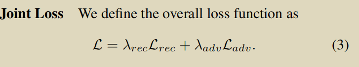
G的loss分三种,传统的foolD的loss,重建的loss,encoder的loss,保证域变换
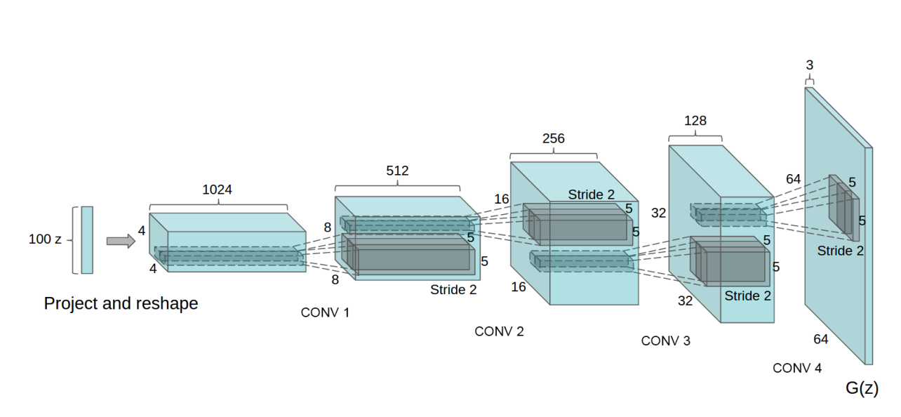
DCGAN
DiscoGAN
跟cyclegan一个东西就是用了两个D
DualGAN
跟DiscoGAN一模一样
EBGAN
ENERGY-BASED GENERATIVE ADVERSARIAL NETWORKS
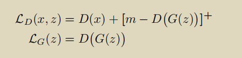
\([·]^+= max(0, ·).\)
当G足够好的时候,就不使用D(G(z))产生的loss了
\(EBGAN-PT\),\(L_G(z)=D_{img}(G(z))+pullaway(D_{embedding}(G(z)))\)

keeping the model from producing samples that are clustered in one or only few modes of pdata.
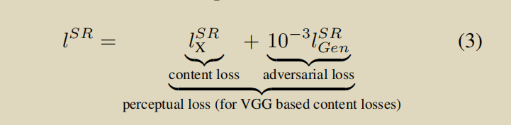
ESRGAN
ESRGAN: Enhanced Super-Resolution Generative Adversarial Networks
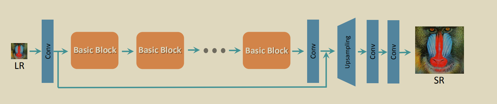

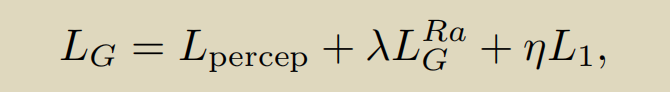
生成器loss的三部分,知觉损失,perceptual loss使用vgg前35层产生的隐藏变量(features before the activation layers 信息更多),衡量fake和real之间的差距。第二个是fool G的loss,第三个是fake和real之间的l1loss.
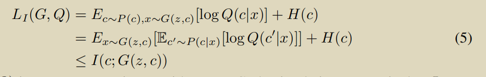
InfoGAN
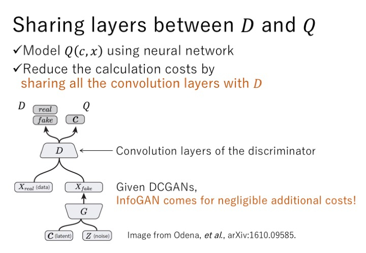
类似acgan
最大化互信息c,和x使得可以通过控制c来控制生成的图片

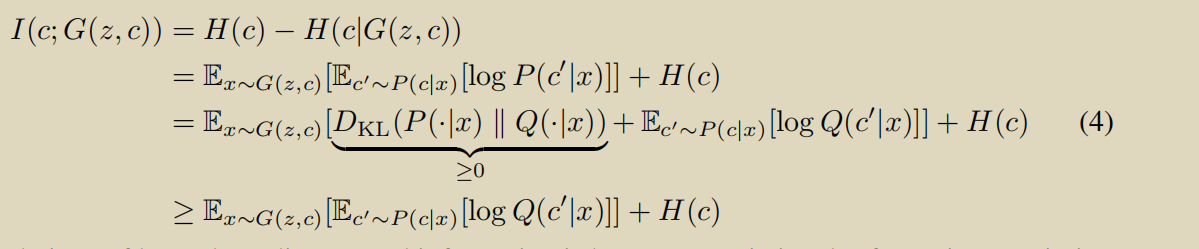
使用辅助分布,\(H(c)\)可以看做是常数
LSGAN
损失函数把交叉熵损失函数改为了最小二乘loss.好处让G尽可能靠近decision boundary
BGAN只对G使用了最小二乘loss,LSGAN对G和D都用了。
MUNIT
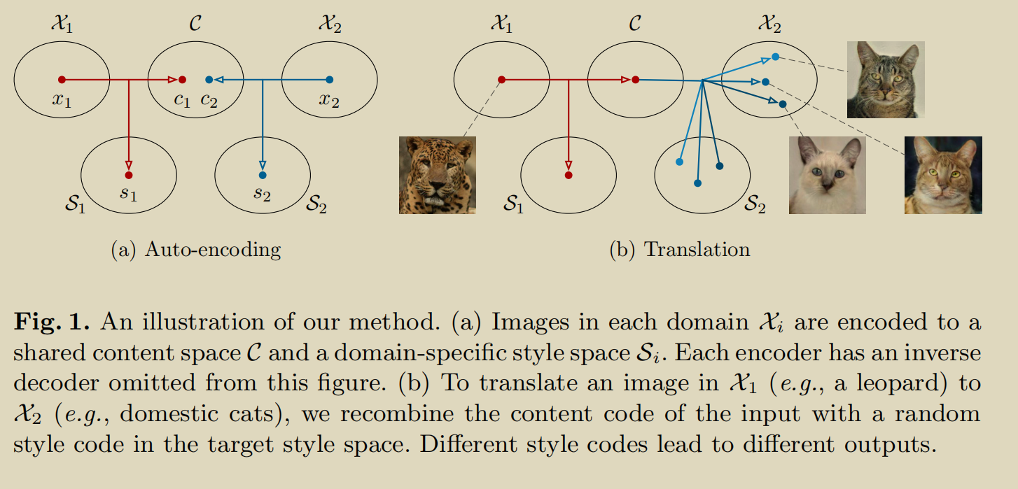
好像就是cyclegan的扩展,多个model多个G,D......
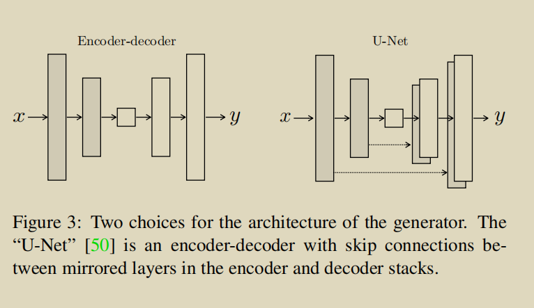
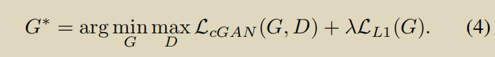
pixel2pixel
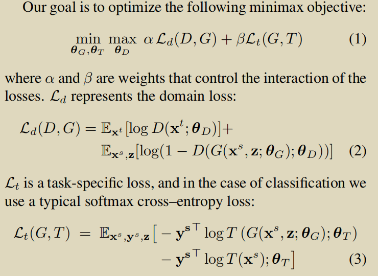
PixelDA

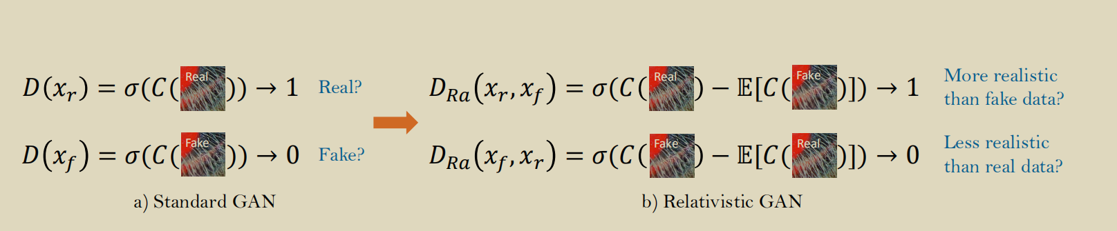
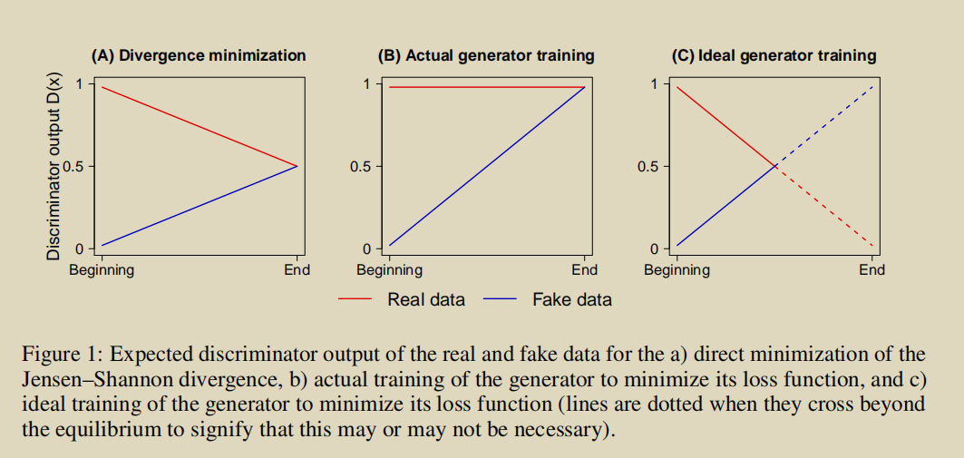
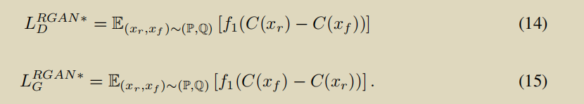
RGAN
The relativistic discriminator: a key element missing from standard GAN
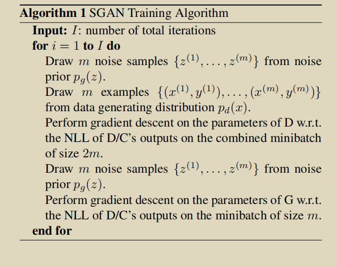
Semi-SurpervisedGAN
Semi-Supervised Learning with Generative Adversarial Networks
D是一个分类器,fake是N+1类数据
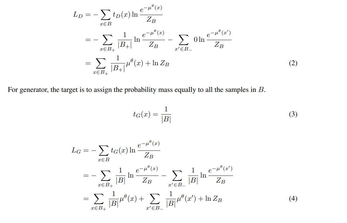
Softmax GAN
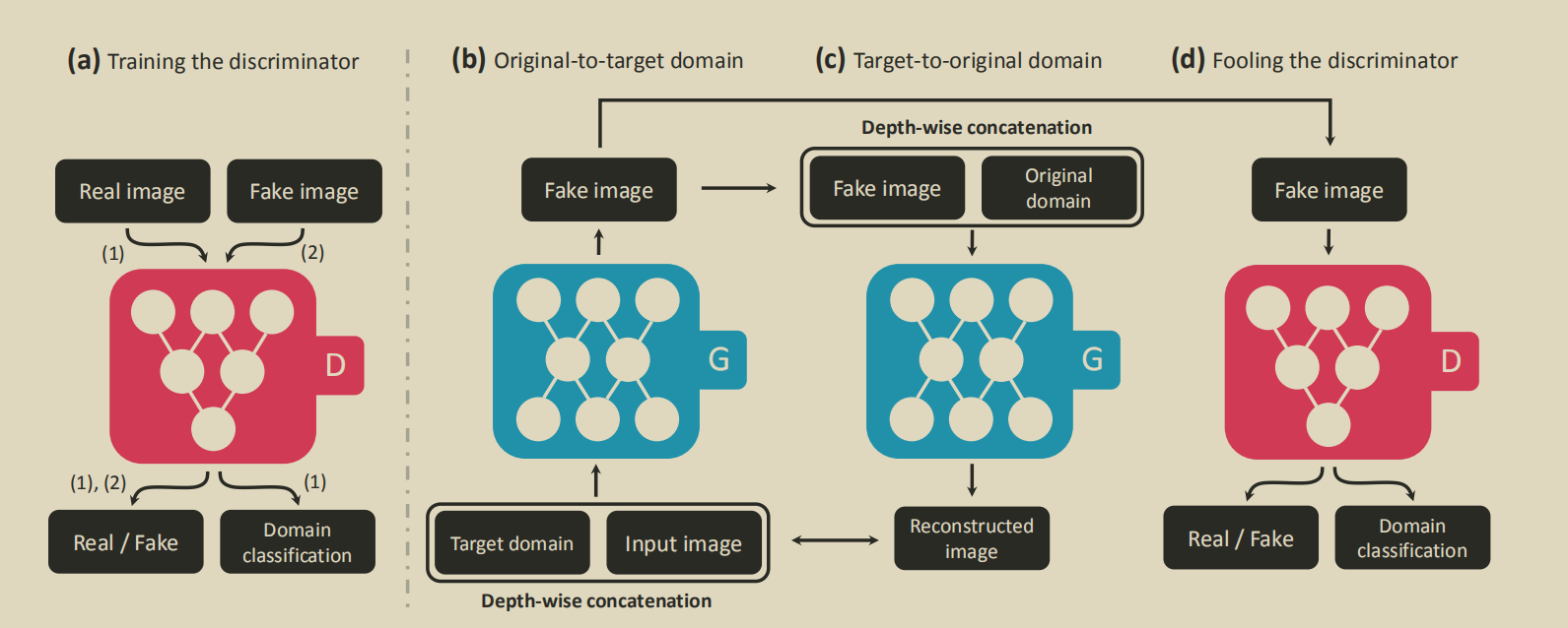
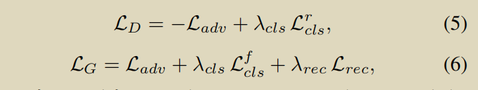
StarGAN
RSGAN

UNIT
跟cogan一样
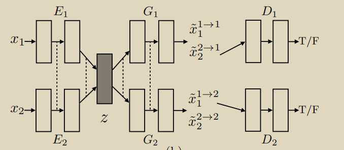
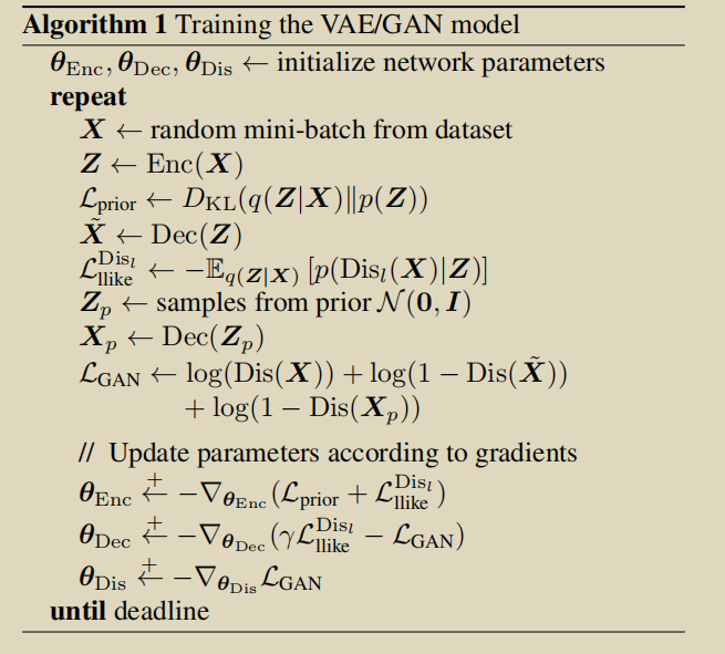
VAEGAN

Wasserstein GAN
GAN的问题


判别器越好,生成器梯度消失越严重
定理:\(p_{data}\)与\(p_g\)的支撑集是高维空间的低维流形(manifold)时,\(p_{data}\)与\(p_g\)重叠部分的测度(measure)为0的概率为1
- 支撑集: 函数非零子集,概率分布的支撑集指所有概率密度非零部分的集合
- 流形: 高维空间中曲线、曲面概念的拓展,如三维空间曲面是二维流形,因为他的本质维度只有2;同理三维空间或二维空间的曲线是一个一维流形
- 测度:超体积
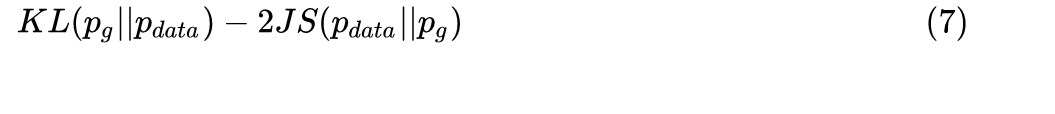
改变的第二种loss不合理
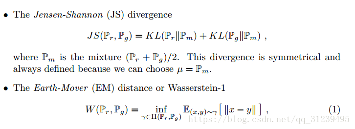
由公式7可以看出来,kl,和js都是衡量分布距离,一正一负,纠结
KL散度是非对称的,\(p_g\rightarrow 0,p_{data}\rightarrow 1\)时,\(KL(p_g||p_{data})\rightarrow 0\),反过来却是\(KL(p_g||p_{data}) \rightarrow \infty\),直观上理解就是,当生成错误样本时,惩罚是巨大的;但是没生成真实样本的惩罚却很小,这样会导致GAN会产生一些重复且惩罚低的样本,而不会产生多样性的样本,导致惩罚很高
用wassertein距离代替kl divergence.


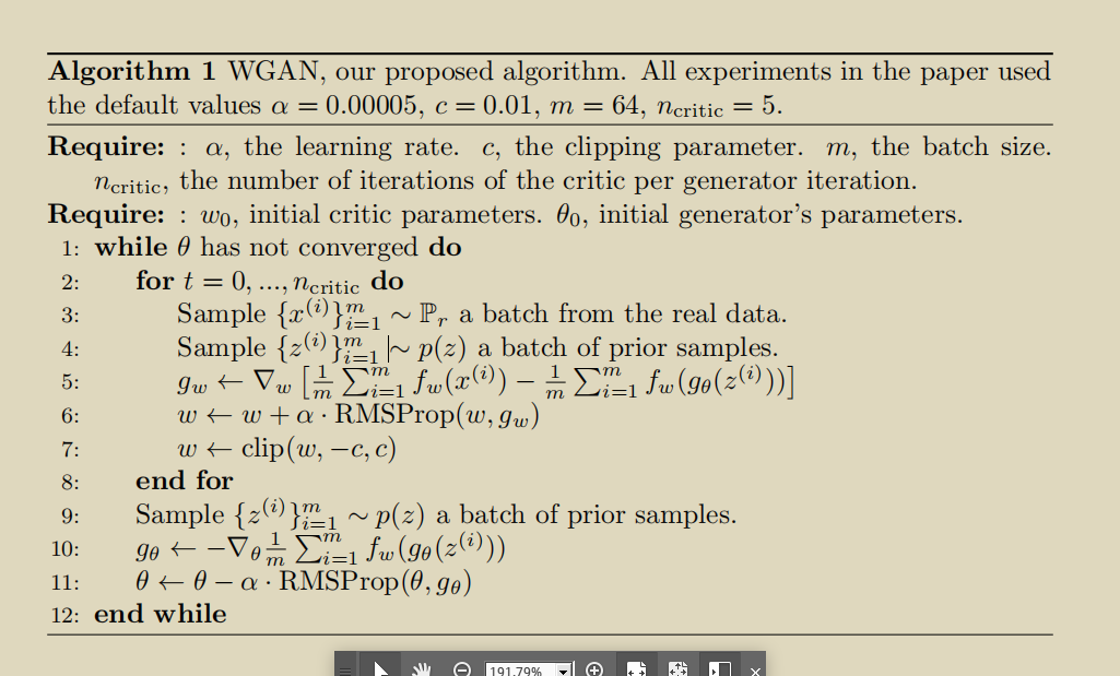
挖了一个L约束的坑,论文中的weight-clip的方法,就是凑上去的。
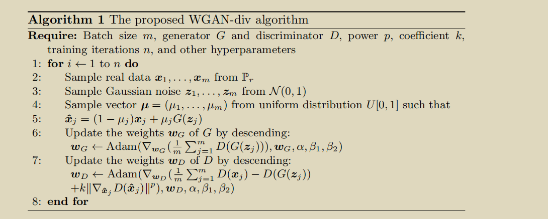
Wassersterin GAN GP
使用了GP的方法

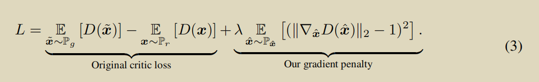
不能在所有样本空间采样计算D(x)的梯度,就用了一个真实样本到采样样本之间插值这样一个区间来采样,进行约束,约束让梯度越接近1越好,实现结果表示很好,缺乏理论支撑。同样存才问题
Wasserseterin GAN DIV