神经网络入门——13实现梯度下降

实现梯度下降

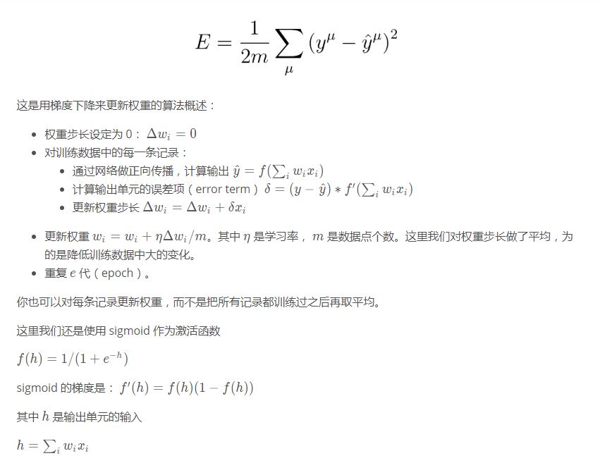
现在我们知道了如何更新我们的权重：

你看到的是如何实现一次更新，那我们如何把代码转化为能够计算多次权重更新，使得我们的网络能够真正学习呢？

作为示例，我们拿一个研究生学院录取数据，用梯度下降训练一个网络。数据可以在这里找到。数据有三个输入特征：GRE 分数、GPA 分数和本科院校排名（从 1 到 4）。排名 1 代表最好，排名 4 代表最差。

 

 

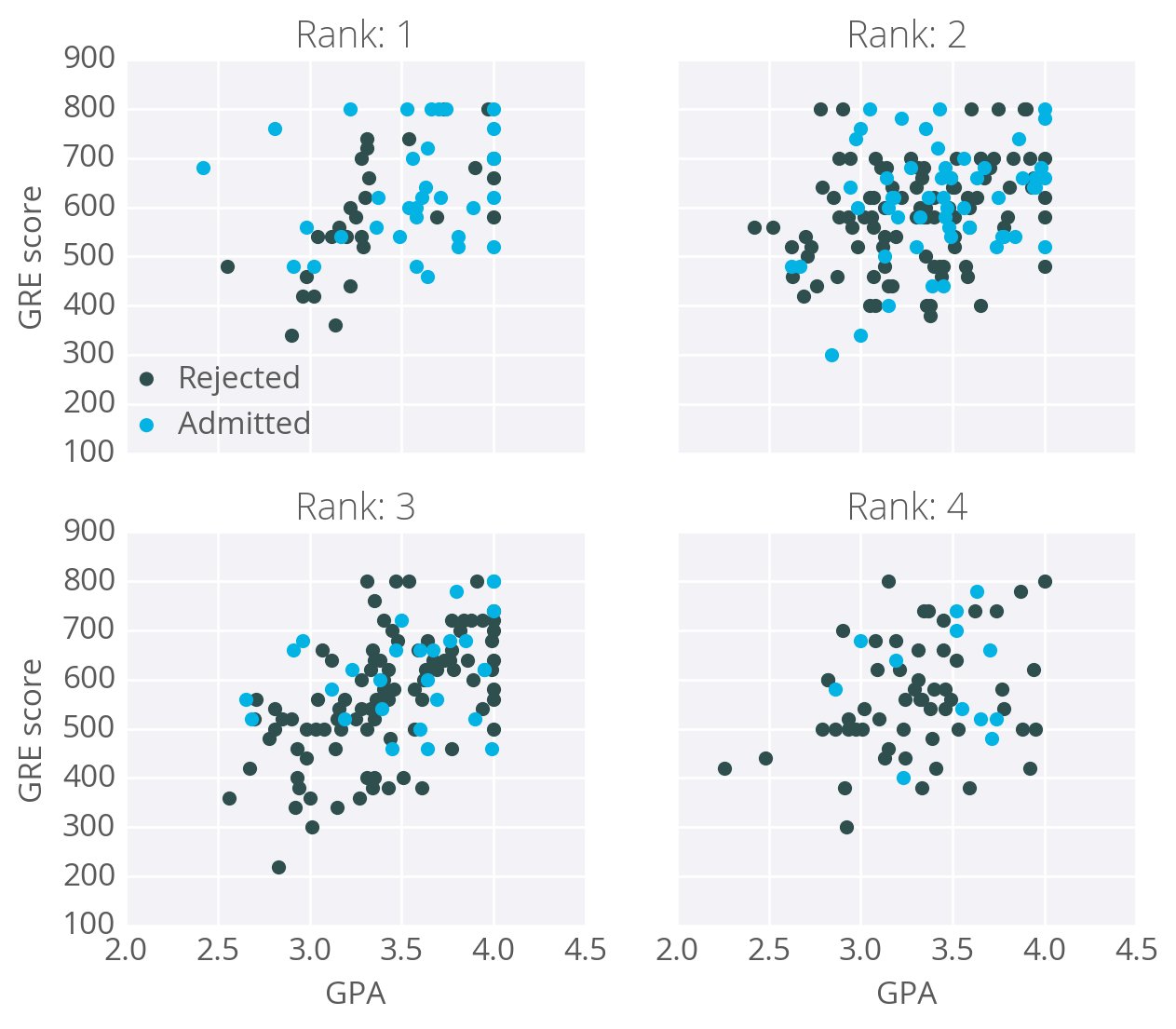
我们的目标是基于这些特征来预测一个学生能否被研究生院录取。这里，我们将使用有一个输出层的网络。用 sigmoid 做为激活函数。

数据清理

你也许认为有三个输入单元，但实际上我们要先做数据转换。rank 是类别特征，其中的数字并不表示任何相对的值。排名第 2 并不是排名第 1 的两倍；排名第 3 也不是排名第 2 的 1.5 倍。因此，我们需要用 dummy variables 来对 rank 进行编码。把数据分成 4 个新列，用 0 或 1 表示。排名为 1 的行对应 rank_1 列的值为 1 ，其余三列的值为 0；排名为 2 的行对应 rank_2 列的值为 1 ，其余三列的值为 0，以此类推。

我们还需要把 GRE 和 GPA 数据标准化，也就是说使得它们的均值为 0，标准偏差为 1。因为 sigmoid 函数会挤压很大或者很小的输入，所以这一步是必要的。很大或者很小输入的梯度为 0，这意味着梯度下降的步长也会是 0。由于 GRE 和 GPA 的值都相当大，我们在初始化权重的时候需要非常小心，否则梯度下降步长将会消失，网络也没法训练了。相对地，如果我们对数据做了标准化处理，就能更容易地对权重进行初始化。

这只是一个简单介绍，你之后还会学到如何预处理数据，如果你想了解我是怎么做的，可以查看下面编程练习中的 data_prep.py 文件。

 

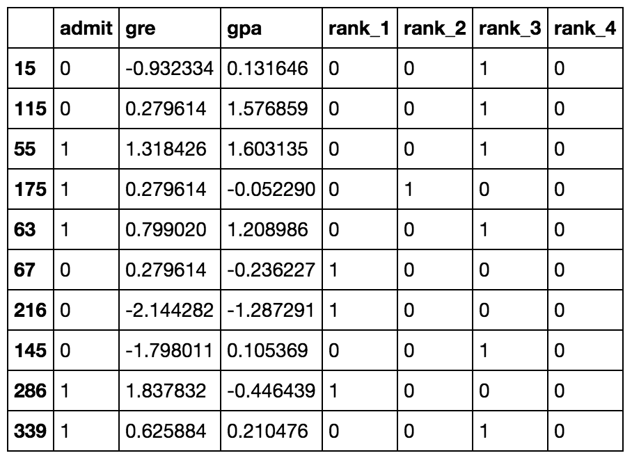
经过转换后的 10 行数据

现在数据已经准备好了，我们看到有六个输入特征：gre、gpa，以及四个 rank 的虚拟变量 （dummy variables）。

均方差

这里我们要对如何计算误差做一点小改变。我们不计算 SSE，而是用误差平方的均值（mean of the square errors，MSE）。现在我们要处理很多数据，把所有权重更新加起来会导致很大的更新，使得梯度下降无法收敛。为了避免这种情况，你需要一个很小的学习率。这里我们还可以除以数据点的数量 mm 来取平均。这样，无论我们有多少数据，我们的学习率通常会在 0.01 to 0.001 之间。我们用 MSE（下图）来计算梯度，结果跟之前一样，只是取了平均而不是取和。

import numpy as np
from data_prep import features, targets, features_test, targets_test


def sigmoid(x):
    """
    Calculate sigmoid
    """
    return 1 / (1 + np.exp(-x))

# TODO: We haven't provided the sigmoid_prime function like we did in
#       the previous lesson to encourage you to come up with a more
#       efficient solution. If you need a hint, check out the comments
#       in solution.py from the previous lecture.

# Use to same seed to make debugging easier
np.random.seed(42)

n_records, n_features = features.shape
last_loss = None

# Initialize weights
weights = np.random.normal(scale=1 / n_features**.5, size=n_features)

# Neural Network hyperparameters
epochs = 1000
learnrate = 0.5

for e in range(epochs):
    del_w = np.zeros(weights.shape)
    for x, y in zip(features.values, targets):
        # Loop through all records, x is the input, y is the target

        # Activation of the output unit
        #   Notice we multiply the inputs and the weights here 
        #   rather than storing h as a separate variable 
        output = sigmoid(np.dot(x, weights))

        # The error, the target minus the network output
        error = y - output

        # The error term
        #   Notice we calulate f'(h) here instead of defining a separate
        #   sigmoid_prime function. This just makes it faster because we
        #   can re-use the result of the sigmoid function stored in
        #   the output variable
        error_term = error * output * (1 - output)

        # The gradient descent step, the error times the gradient times the inputs
        del_w += error_term * x

    # Update the weights here. The learning rate times the 
    # change in weights, divided by the number of records to average
    weights += learnrate * del_w / n_records

    # Printing out the mean square error on the training set
    if e % (epochs / 10) == 0:
        out = sigmoid(np.dot(features, weights))
        loss = np.mean((out - targets) ** 2)
        if last_loss and last_loss < loss:
            print("Train loss: ", loss, "  WARNING - Loss Increasing")
        else:
            print("Train loss: ", loss)
        last_loss = loss


# Calculate accuracy on test data
tes_out = sigmoid(np.dot(features_test, weights))
predictions = tes_out > 0.5
accuracy = np.mean(predictions == targets_test)
print("Prediction accuracy: {:.3f}".format(accuracy))

import numpy as np
import pandas as pd

admissions = pd.read_csv('binary.csv')

# Make dummy variables for rank
data = pd.concat([admissions, pd.get_dummies(admissions['rank'], prefix='rank')], axis=1)
data = data.drop('rank', axis=1)

# Standarize features
for field in ['gre', 'gpa']:
    mean, std = data[field].mean(), data[field].std()
    data.loc[:,field] = (data[field]-mean)/std
    
# Split off random 10% of the data for testing
np.random.seed(42)
sample = np.random.choice(data.index, size=int(len(data)*0.9), replace=False)
data, test_data = data.ix[sample], data.drop(sample)

# Split into features and targets
features, targets = data.drop('admit', axis=1), data['admit']
features_test, targets_test = test_data.drop('admit', axis=1), test_data['admit']

admit,gre,gpa,rank
0,380,3.61,3
1,660,3.67,3
1,800,4,1
1,640,3.19,4
0,520,2.93,4
1,760,3,2
1,560,2.98,1
0,400,3.08,2
1,540,3.39,3
0,700,3.92,2
0,800,4,4
0,440,3.22,1
1,760,4,1
0,700,3.08,2
1,700,4,1
0,480,3.44,3
0,780,3.87,4
0,360,2.56,3
0,800,3.75,2
1,540,3.81,1
0,500,3.17,3
1,660,3.63,2
0,600,2.82,4
0,680,3.19,4
1,760,3.35,2
1,800,3.66,1
1,620,3.61,1
1,520,3.74,4
1,780,3.22,2
0,520,3.29,1
0,540,3.78,4
0,760,3.35,3
0,600,3.4,3
1,800,4,3
0,360,3.14,1
0,400,3.05,2
0,580,3.25,1
0,520,2.9,3
1,500,3.13,2
1,520,2.68,3
0,560,2.42,2
1,580,3.32,2
1,600,3.15,2
0,500,3.31,3
0,700,2.94,2
1,460,3.45,3
1,580,3.46,2
0,500,2.97,4
0,440,2.48,4
0,400,3.35,3
0,640,3.86,3
0,440,3.13,4
0,740,3.37,4
1,680,3.27,2
0,660,3.34,3
1,740,4,3
0,560,3.19,3
0,380,2.94,3
0,400,3.65,2
0,600,2.82,4
1,620,3.18,2
0,560,3.32,4
0,640,3.67,3
1,680,3.85,3
0,580,4,3
0,600,3.59,2
0,740,3.62,4
0,620,3.3,1
0,580,3.69,1
0,800,3.73,1
0,640,4,3
0,300,2.92,4
0,480,3.39,4
0,580,4,2
0,720,3.45,4
0,720,4,3
0,560,3.36,3
1,800,4,3
0,540,3.12,1
1,620,4,1
0,700,2.9,4
0,620,3.07,2
0,500,2.71,2
0,380,2.91,4
1,500,3.6,3
0,520,2.98,2
0,600,3.32,2
0,600,3.48,2
0,700,3.28,1
1,660,4,2
0,700,3.83,2
1,720,3.64,1
0,800,3.9,2
0,580,2.93,2
1,660,3.44,2
0,660,3.33,2
0,640,3.52,4
0,480,3.57,2
0,700,2.88,2
0,400,3.31,3
0,340,3.15,3
0,580,3.57,3
0,380,3.33,4
0,540,3.94,3
1,660,3.95,2
1,740,2.97,2
1,700,3.56,1
0,480,3.13,2
0,400,2.93,3
0,480,3.45,2
0,680,3.08,4
0,420,3.41,4
0,360,3,3
0,600,3.22,1
0,720,3.84,3
0,620,3.99,3
1,440,3.45,2
0,700,3.72,2
1,800,3.7,1
0,340,2.92,3
1,520,3.74,2
1,480,2.67,2
0,520,2.85,3
0,500,2.98,3
0,720,3.88,3
0,540,3.38,4
1,600,3.54,1
0,740,3.74,4
0,540,3.19,2
0,460,3.15,4
1,620,3.17,2
0,640,2.79,2
0,580,3.4,2
0,500,3.08,3
0,560,2.95,2
0,500,3.57,3
0,560,3.33,4
0,700,4,3
0,620,3.4,2
1,600,3.58,1
0,640,3.93,2
1,700,3.52,4
0,620,3.94,4
0,580,3.4,3
0,580,3.4,4
0,380,3.43,3
0,480,3.4,2
0,560,2.71,3
1,480,2.91,1
0,740,3.31,1
1,800,3.74,1
0,400,3.38,2
1,640,3.94,2
0,580,3.46,3
0,620,3.69,3
1,580,2.86,4
0,560,2.52,2
1,480,3.58,1
0,660,3.49,2
0,700,3.82,3
0,600,3.13,2
0,640,3.5,2
1,700,3.56,2
0,520,2.73,2
0,580,3.3,2
0,700,4,1
0,440,3.24,4
0,720,3.77,3
0,500,4,3
0,600,3.62,3
0,400,3.51,3
0,540,2.81,3
0,680,3.48,3
1,800,3.43,2
0,500,3.53,4
1,620,3.37,2
0,520,2.62,2
1,620,3.23,3
0,620,3.33,3
0,300,3.01,3
0,620,3.78,3
0,500,3.88,4
0,700,4,2
1,540,3.84,2
0,500,2.79,4
0,800,3.6,2
0,560,3.61,3
0,580,2.88,2
0,560,3.07,2
0,500,3.35,2
1,640,2.94,2
0,800,3.54,3
0,640,3.76,3
0,380,3.59,4
1,600,3.47,2
0,560,3.59,2
0,660,3.07,3
1,400,3.23,4
0,600,3.63,3
0,580,3.77,4
0,800,3.31,3
1,580,3.2,2
1,700,4,1
0,420,3.92,4
1,600,3.89,1
1,780,3.8,3
0,740,3.54,1
1,640,3.63,1
0,540,3.16,3
0,580,3.5,2
0,740,3.34,4
0,580,3.02,2
0,460,2.87,2
0,640,3.38,3
1,600,3.56,2
1,660,2.91,3
0,340,2.9,1
1,460,3.64,1
0,460,2.98,1
1,560,3.59,2
0,540,3.28,3
0,680,3.99,3
1,480,3.02,1
0,800,3.47,3
0,800,2.9,2
1,720,3.5,3
0,620,3.58,2
0,540,3.02,4
0,480,3.43,2
1,720,3.42,2
0,580,3.29,4
0,600,3.28,3
0,380,3.38,2
0,420,2.67,3
1,800,3.53,1
0,620,3.05,2
1,660,3.49,2
0,480,4,2
0,500,2.86,4
0,700,3.45,3
0,440,2.76,2
1,520,3.81,1
1,680,2.96,3
0,620,3.22,2
0,540,3.04,1
0,800,3.91,3
0,680,3.34,2
0,440,3.17,2
0,680,3.64,3
0,640,3.73,3
0,660,3.31,4
0,620,3.21,4
1,520,4,2
1,540,3.55,4
1,740,3.52,4
0,640,3.35,3
1,520,3.3,2
1,620,3.95,3
0,520,3.51,2
0,640,3.81,2
0,680,3.11,2
0,440,3.15,2
1,520,3.19,3
1,620,3.95,3
1,520,3.9,3
0,380,3.34,3
0,560,3.24,4
1,600,3.64,3
1,680,3.46,2
0,500,2.81,3
1,640,3.95,2
0,540,3.33,3
1,680,3.67,2
0,660,3.32,1
0,520,3.12,2
1,600,2.98,2
0,460,3.77,3
1,580,3.58,1
1,680,3,4
1,660,3.14,2
0,660,3.94,2
0,360,3.27,3
0,660,3.45,4
0,520,3.1,4
1,440,3.39,2
0,600,3.31,4
1,800,3.22,1
1,660,3.7,4
0,800,3.15,4
0,420,2.26,4
1,620,3.45,2
0,800,2.78,2
0,680,3.7,2
0,800,3.97,1
0,480,2.55,1
0,520,3.25,3
0,560,3.16,1
0,460,3.07,2
0,540,3.5,2
0,720,3.4,3
0,640,3.3,2
1,660,3.6,3
1,400,3.15,2
1,680,3.98,2
0,220,2.83,3
0,580,3.46,4
1,540,3.17,1
0,580,3.51,2
0,540,3.13,2
0,440,2.98,3
0,560,4,3
0,660,3.67,2
0,660,3.77,3
1,520,3.65,4
0,540,3.46,4
1,300,2.84,2
1,340,3,2
1,780,3.63,4
1,480,3.71,4
0,540,3.28,1
0,460,3.14,3
0,460,3.58,2
0,500,3.01,4
0,420,2.69,2
0,520,2.7,3
0,680,3.9,1
0,680,3.31,2
1,560,3.48,2
0,580,3.34,2
0,500,2.93,4
0,740,4,3
0,660,3.59,3
0,420,2.96,1
0,560,3.43,3
1,460,3.64,3
1,620,3.71,1
0,520,3.15,3
0,620,3.09,4
0,540,3.2,1
1,660,3.47,3
0,500,3.23,4
1,560,2.65,3
0,500,3.95,4
0,580,3.06,2
0,520,3.35,3
0,500,3.03,3
0,600,3.35,2
0,580,3.8,2
0,400,3.36,2
0,620,2.85,2
1,780,4,2
0,620,3.43,3
1,580,3.12,3
0,700,3.52,2
1,540,3.78,2
1,760,2.81,1
0,700,3.27,2
0,720,3.31,1
1,560,3.69,3
0,720,3.94,3
1,520,4,1
1,540,3.49,1
0,680,3.14,2
0,460,3.44,2
1,560,3.36,1
0,480,2.78,3
0,460,2.93,3
0,620,3.63,3
0,580,4,1
0,800,3.89,2
1,540,3.77,2
1,680,3.76,3
1,680,2.42,1
1,620,3.37,1
0,560,3.78,2
0,560,3.49,4
0,620,3.63,2
1,800,4,2
0,640,3.12,3
0,540,2.7,2
0,700,3.65,2
1,540,3.49,2
0,540,3.51,2
0,660,4,1
1,480,2.62,2
0,420,3.02,1
1,740,3.86,2
0,580,3.36,2
0,640,3.17,2
0,640,3.51,2
1,800,3.05,2
1,660,3.88,2
1,600,3.38,3
1,620,3.75,2
1,460,3.99,3
0,620,4,2
0,560,3.04,3
0,460,2.63,2
0,700,3.65,2
0,600,3.89,3