TensorFlow良心入门教程

All the matrials come from Machine Learning class in Polyu,HK and I reorganize them and add reference materials.I promise that I only use them to study and non-proft

.ipynb源文件可通过我的onedrive下载：https://1drv.ms/u/s!Al86h1dThXMNxF-J7FKHKTPkf5yr?e=SAgALh

---

Warm up

A short example for Tensorflow:

import tensorflow as tf

node1=tf.placeholder(tf.float32)
node2=tf.placeholder(tf.float32)
node3=tf.add(node1,node2)
tf.Session().run(node3,{node1:4,node2:4})

8.0

Basic ideas

It's okay if you don't understand the content well in this section.Section 3rd will be much more detailed and basic

Core TensorFlow constructs

• Dataflow Graphs: entire computation
• Data Nodes: individual data or operations
• Edges: implicit dependencies between nodes
• Operations: any computation
• Constants: single values (tensors)

Choose the place to run code

The whole point of having a dataflow representation is flexibility in choosing location. Tensorflow lets you choose the device to run the code:

Computational graph

A TensorFlow Core programs contains two sections:
Building the computational graph.
Running the computational graph.

So what is a computational graph?

A computational graph is a series of TensorFlow operations arranged into a graph of nodes.

Node

Each node takes zero or more tensors as inputs and produces a tensor as an output.The type of node could be constant,variable,operations and so on.

All nodes return tensors, or higher-dimensional matrices

Tensor

A tensor consists of a set of primitive(原始) values shaped into an array of any number of dimensions. 

Variable

To make the model trainable, we need to be able to modify the graph to get new outputs with the same input.So we should use variable:

Variables allow us to add trainable parameters to a graph.They are constructed with a type and initial value.

Placeholder

A placeholder is a promise to provide a value later.

Initializer

To initialize all the variables in a TensorFlow program, tf.global_variables_initializer() is needed.

Model Evaluation and Training

To evaluate the model on training data: loss function

TensorFlow provides optimizers that slowly change each variable in order to minimize the loss function. (In the following example we use gradient descent.)

Session(会话)

To actually evaluate the nodes, we must run the computational graph within a session.

A session encapsulates(封装) the control and state of the TensorFlow runtime.

---

A linear Rgression Example:

import numpy as np
# Model parameters
W = tf.Variable([.3], dtype=tf.float32)
b = tf.Variable([-.3], dtype=tf.float32)
#Model input and output
x = tf.placeholder(tf.float32)
linear_model = W * x + b #Operator Overloading!
y=tf.placeholder(tf.float32)
#loss
loss=tf.reduce_sum(tf.square(linear_model-y))
#optimizer
optimizer=tf.train.GradientDescentOptimizer(0.01)
train=optimizer.minimize(loss)
#training data
X_train=[1,2,3,4]
y_train=[0,-1,-2,-3]
#training loop
init = tf.global_variables_initializer()
with tf.Session() as sess:
    sess.run(init)
    for i in range(1000):
        sess.run(train,{x:X_train,y:y_train})
    #evaluate training accuracy
    curr_W,curr_b,curr_loss=sess.run([W,b,loss],{x:X_train,y:y_train})
print("W:%s b:%s loss:%s"%(curr_W,curr_b,curr_loss))

W:[-0.9999969] b:[0.9999908] loss:5.6999738e-11

Suggested System Design

Parameter server

it focus:

• Hold Mutable state
• Apply updates
• Maintain availability
• Group Name: ps

Worker

it focus:

• Perform “active” actions
• Checkpoint state to FS
• Mostly stateless; can be restarted
• Group name: worker

The implemnetation of TensorFlow

Distributed Master: compiles the graph, including specialization. Think of it kind of like a query optimizer, but honestly it’s really an impoverished compiler Dataflow executor: the scheduler and coordinator, responsible for invoking kernels on various devices.

---

Detailed understanding

Introducing Tensors

---

The term "tensor" in ML,especially tensorflow, has no relation with the term "tensor(called 张量 in Chinese" in physics!

I attach a link which introduces the tensor used in physics and mathematics.After reading it you will find out that maybe google misuse the "tensor"

---

To understand tensors well, it’s good to have some working knowledge of linear algebra and vector calculus. You already read in the introduction that tensors are implemented in TensorFlow as multidimensional data arrays, but some more introduction is maybe needed in order to completely grasp tensors and their use in machine learning.

Plane Vectors(平面向量)

Please be aware that the content in this section is very very simple
Before you go into plane vectors, it’s a good idea to shortly revise the concept of “vectors”; Vectors are special types of matrices, which are rectangular arrays of numbers. Because vectors are ordered collections of numbers, they are often seen as column matrices(列向量): they have just one column and a certain number of rows. In other terms, you could also consider vectors as scalar(标量) magnitudes that have been given a direction.

Remember: an example of a scalar is “5 meters” or “60 m/sec”, while a vector is, for example, “5 meters north” or “60 m/sec East”. The difference between these two is obviously that the vector has a direction. Nevertheless, these examples that you have seen up until now might seem far off from the vectors that you might encounter when you’re working with machine learning problems. This is normal; The length of a mathematical vector is a pure number: it is absolute. The direction, on the other hand, is relative: it is measured relative to some reference direction and has units of radians or degrees. You usually assume that the direction is positive and in counterclockwise rotation from the reference direction.

Visually, of course, you represent vectors as arrows, as you can see in the picture above. This means that you can consider vectors also as arrows that have direction and length. The direction is indicated by the arrow’s head, while the length is indicated by the length of the arrow.

So what about plane vectors then?

Plane vectors are the most straightforward setup of tensors. They are much like regular vectors as you have seen above, with the sole difference that they find themselves in a vector space. To understand this better, let’s start with an example: you have a vector that is 2 X 1. This means that the vector belongs to the set of real numbers that come paired two at a time. Or, stated differently, they are part of two-space. In such cases, you can represent vectors on the coordinate (x,y) plane with arrows or rays.

Working from this coordinate(坐标) plane in a standard position where vectors have their endpoint at the origin (0,0), you can derive the x coordinate by looking at the first row of the vector, while you’ll find the y coordinate in the second row. Of course, this standard position doesn’t always need to be maintained: vectors can move parallel to themselves in the plane without experiencing changes.

Note that similarly, for vectors that are of size 3 X 1, you talk about the three-space. You can represent the vector as a three-dimensional figure with arrows pointing to positions in the vectors pace: they are drawn on the standard x, y and z axes.

It’s nice to have these vectors and to represent them on the coordinate plane, but in essence(本质), you have these vectors so that you can perform operations on them and one thing that can help you in doing this is by expressing your vectors as bases or unit vectors(单位向量).

Unit vectors are vectors with a magnitude(大小) of one. You’ll often recognize the unit vector by a lowercase letter with a circumflex, or “hat”. Unit vectors will come in convenient if you want to express a 2-D or 3-D vector as a sum of two or three orthogonal components, such as the x− and y−axes, or the z−axis.

And when you are talking about expressing one vector, for example, as sums of components, you’ll see that you’re talking about component vectors, which are two or more vectors whose sum is that given vector.

(now the very very easy part ends)

---

Tensors

Next to plane vectors, also covectors and linear operators are two other cases that all three together have one thing in common: they are specific cases of tensors. You still remember how a vector was characterized in the previous section as scalar magnitudes that have been given a direction. A tensor, then, is the mathematical representation of a physical entity that may be characterized by magnitude and multiple directions.

And, just like you represent a scalar with a single number and a vector with a sequence of three numbers in a 3-dimensional space, for example, a tensor can be represented by an array of 3^R numbers in a 3-dimensional space.

The “R” in this notation represents the rank of the tensor: this means that in a 3-dimensional space, a second-rank tensor can be represented by 3 to the power of 2 or 9 numbers. In an N-dimensional space, scalars will still require only one number, while vectors will require N numbers, and tensors will require N^R numbers. This explains why you often hear that scalars are tensors of rank 0: since they have no direction, you can represent them with one number.

With this in mind, it’s relatively easy to recognize scalars, vectors, and tensors and to set them apart: scalars can be represented by a single number, vectors by an ordered set of numbers, and tensors by an array of numbers.

What makes tensors so unique is the combination of components and basis vectors(向量基): basis vectors transform one way between reference frames and the components transform in just such a way as to keep the combination between components and basis vectors the same.

---

This article introduce the "sensor" in physics and mathematics:
source:https://www.jianshu.com/p/2a0f7f7735ad

And this picture summary what is sensor in tensorflow:

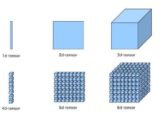
So the sensor in ML actually is just a kind of Multidimensional Arrays

---

Getting Started With TensorFlow: Basics

You’ll generally write TensorFlow programs, which you run as a chunk; This is at first sight kind of contradictory when you’re working with Python. However, if you would like, you can also use TensorFlow’s Interactive Session, which you can use to work more interactively with the library. This is especially handy when you’re used to working with IPython.

For this tutorial, you’ll focus on the second option: this will help you to get kickstarted with deep learning in TensorFlow. But before you go any further into this, let’s first try out some minor stuff before you start with the heavy lifting.

First, import the tensorflow library under the alias(别名) tf, as you have seen in the previous section. Then initialize two variables that are actually constants. Pass an array of four numbers to the constant() function.

Note that you could potentially also pass in an integer, but that more often than not, you’ll find yourself working with arrays. As you saw in the introduction, tensors are all about arrays! So make sure that you pass in an array :) Next, you can use multiply() to multiply your two variables. Store the result in the result variable. Lastly, print out the result with the help of the print() function.

# Import `tensorflow`
import tensorflow as tf

# Initialize two constants
#we usually work with array not integer
x1 = tf.constant([1,2,3,4])
x2 = tf.constant([5,6,7,8])

# Multiply
result = tf.multiply(x1, x2)

# Print the result
print(result)

Tensor("Mul_7:0", shape=(4,), dtype=int32)

Note that you have defined constants above. However, there are two other types of values that you can potentially use, namely placeholders, which are values that are unassigned and that will be initialized by the session when you run it. Like the name already gave away, it’s just a placeholder for a tensor that will always be fed when the session is run; There are also Variables, which are values that can change. The constants, as you might have already gathered, are values that don’t change.

The result of the lines of code is an abstract tensor in the computation graph. However, contrary to what you might expect, the result doesn’t actually get calculated. It just defined the model, but no process ran to calculate the result. You can see this in the print-out: there’s not really a result that you want to see (namely, 30). This means that TensorFlow has a lazy evaluation!

However, if you do want to see the result, you have to run this code in an interactive session. You can do this in a few ways, as is demonstrated below:

# Intialize the Session
sess = tf.Session()

# Print the result
print(sess.run(result))

# Close the session
sess.close()

[ 5 12 21 32]

Note that you can also use the following lines of code to start up an interactive Session, run the result and close the Session automatically again after printing the output:

# Initialize Session and run `result`
#the "with" method will close the session automatically
with tf.Session() as sess:
  output = sess.run(result)
  print(output)

[ 5 12 21 32]

First Neural Network:Basic Classification

This tutorial trains a neural network model to classify images of clothing, like sneakers and shirts. It's okay if you don't understand all the details, this is a fast-paced overview of a complete TensorFlow program with the details explained as we go.

This tutorial uses tf.keras, a high-level API to build and train models in TensorFlow.

from __future__ import absolute_import, division, print_function

# TensorFlow and tf.keras
import tensorflow as tf
from tensorflow import keras

# Helper libraries
import numpy as np
import matplotlib.pyplot as plt

print(tf.__version__)

1.14.0

Import the Fashion MNIST dataset

This tutorial uses the Fashion MNIST dataset which contains 70,000 grayscale images in 10 categories. The images show individual articles of clothing at low resolution (28 by 28 pixels).

We will use 60,000 images to train the network and 10,000 images to evaluate how accurately the network learned to classify images. You can access the Fashion MNIST directly from TensorFlow, just import and load the data:

fashion_mnist = keras.datasets.fashion_mnist

(train_images, train_labels), (test_images, test_labels) = fashion_mnist.load_data()

Downloading data from https://storage.googleapis.com/tensorflow/tf-keras-datasets/train-labels-idx1-ubyte.gz
32768/29515 [=================================] - 0s 0us/step
Downloading data from https://storage.googleapis.com/tensorflow/tf-keras-datasets/train-images-idx3-ubyte.gz
26427392/26421880 [==============================] - 3s 0us/step
Downloading data from https://storage.googleapis.com/tensorflow/tf-keras-datasets/t10k-labels-idx1-ubyte.gz
8192/5148 [===============================================] - 0s 0us/step
Downloading data from https://storage.googleapis.com/tensorflow/tf-keras-datasets/t10k-images-idx3-ubyte.gz
4423680/4422102 [==============================] - 1s 0us/step

# show the type and size 
print(type(train_images),train_images.size)

<class 'numpy.ndarray'> 47040000

Loading the dataset returns four NumPy arrays:

The train_images and train_labels arrays are the training set—the data the model uses to learn.

The model is tested against the test set, the test_images, and test_labels arrays.

The images are 28x28 NumPy arrays, with pixel values ranging between 0 and 255.(yes,no color,just grayscale value) The labels are an array of integers, ranging from 0 to 9. These correspond to the class of clothing the image represents:

• 0 - T-shirt/top
• 1 - Trouser
• 2 - Pullover
• 3 - Dress
• 4 - Coat
• 5 - Sandal
• 6 - Shirt
• 7 - Sneaker
• 8 - Bag
• 9 - Ankle boot

Each image is mapped to a single label. Since the class names are not included with the dataset, store them here to use later when plotting the images:

class_names = ['T-shirt/top', 'Trouser', 'Pullover', 'Dress', 'Coat', 
               'Sandal', 'Shirt', 'Sneaker', 'Bag', 'Ankle boot']

Explore the data

Let's explore the format of the dataset before training the model. The following shows there are 60,000 images in the training set, with each image represented as 28 x 28 pixels:

train_images.shape

(60000, 28, 28)

Likewise, there are 60,000 labels in the training set:

len(train_labels)

60000

Each label is an integer between 0 and 9:

train_labels

array([9, 0, 0, ..., 3, 0, 5], dtype=uint8)

Preprocess the data

The data must be preprocessed before training the network. If you inspect the first image in the training set, you will see that the pixel values fall in the range of 0 to 255:

plt.figure()
plt.imshow(train_images[0])
plt.colorbar()
plt.grid(False)
plt.show()

We scale these values to a range of 0 to 1 before feeding to the neural network model. For this, we divide the values by 255. It's important that the training set and the testing set are preprocessed in the same way:

plt.figure(figsize=(10,10))
for i in range(25):
    plt.subplot(5,5,i+1)#plot the (i+1)th picture
    plt.xticks([])
    plt.yticks([])
    plt.grid(False)
    plt.imshow(train_images[i], cmap=plt.cm.binary)
    plt.xlabel(class_names[train_labels[i]])
plt.show()

What is "cmap" in the plt command:

cmap: 颜色图谱（colormap), 默认绘制为RGB(A)颜色空间。plt.cm.binary是使用灰度显示

Build the model

Building the neural network requires configuring the layers of the model, then compiling the model.

Setup the layers

The basic building block of a neural network is the layer. Layers extract representations from the data fed into them. And, hopefully, these representations are more meaningful for the problem at hand.

Most of deep learning consists of chaining together simple layers. Most layers, like tf.keras.layers.Dense, have parameters that are learned during training.

model = keras.Sequential([
    keras.layers.Flatten(input_shape=(28, 28)),
    keras.layers.Dense(128, activation=tf.nn.relu),
    keras.layers.Dense(10, activation=tf.nn.softmax)
])

WARNING:tensorflow:From /home/jiading/.conda/envs/nn/lib/python3.7/site-packages/tensorflow/python/ops/init_ops.py:1251: calling VarianceScaling.__init__ (from tensorflow.python.ops.init_ops) with dtype is deprecated and will be removed in a future version.
Instructions for updating:
Call initializer instance with the dtype argument instead of passing it to the constructor

The first layer in this network, tf.keras.layers.Flatten, transforms the format of the images from a 2d-array (of 28 by 28 pixels), to a 1d-array of 28 * 28 = 784 pixels. Think of this layer as unstacking rows of pixels in the image and lining them up. This layer has no parameters to learn; it only reformats the data.

After the pixels are flattened, the network consists of a sequence of two tf.keras.layers.Dense layers. These are densely-connected, or fully-connected, neural layers. The first Dense layer has 128 nodes (or neurons). The second (and last) layer is a 10-node softmax layer—this returns an array of 10 probability scores that sum to 1. Each node contains a score that indicates the probability that the current image belongs to one of the 10 classes.

未完待续，先睡了