JAVA 深度学习-TensorFlow 完整的TensorFlow入门教程

1：你想要学习 TensorFlow，首先你得安装Tensorflow，在你学习的时候你最好懂以下的知识：

    a：怎么用python编程；

     b：了解一些关于数组的知识；

     c：最理想的情况是：关于机器学习，懂一点点；或者不懂也是可以慢慢开始学习的。

2：TensorFlow提供很多API，最低级别是API: TensorFlow Core，提供给你完成程序控制,还有一些 高级别的API，它们是构建在

TensorFlow Core 之上 的，这些高级别的API更加容易学习和使用， 于此同时，这些高级别的API使得重复的训练任务更加容易，

也使得多个使用者操作对他保持 一致 性， 一个高级别的API像 tf.estimator 帮助你管理数据集合，估量，训练和推理。

3： Tensors TensorFlow的数据中央控制单元是 tensor(张量)，一个tensor由一系列的原始值 组成，这些值被形成一个任意维数的数组。

一个tensor的 列就是它的维度。

4：

import tensorflow as tf
   
   

上面的是TensorFlow 程序典型的导入语句，作用是：赋予Python访问TensorFlow类(classes)，方法（methods），符号(symbols)

5 ： The Computational Graph TensorFlow核心程序由2个独立部分组成：

    a:Building the computational graph构建计算图

    b:Running the computational graph运行计算图

一个computational graph(计算图)是一系列的TensorFlow操作排列成一个节点图。

   
   
node1 = tf.constant( 3.0, dtype=tf.float32)
node2 = tf.constant( 4.0) # also tf.float32 implicitly
print(node1, node2)
   
   

最后打印结果是：

Tensor("Const:0", shape=(), dtype=float32) Tensor("Const_1:0",shape=(), dtype=float32)
   
   

要想打印最终结果，我们必须用到 session:一个session封装了TensorFlow运行时的控制和状态

   
   
sess = tf.Session()
print(sess.run([node1, node2]))
   
   

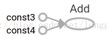
我们可以组合Tensor节点操作(操作仍然是一个节点)来构造更加复杂的计算，

   
   
node3 = tf.add(node1, node2)
print( "node3:", node3)
print( "sess.run(node3):", sess.run(node3))
   
   

打印结果是：

   
   
node3:Tensor( "Add:0", shape=(), dtype=float32)
sess.run(node3): 7.0
   
   

6：TensorFlow提供一个统一的调用称之为 TensorBoard，它能展示一个计算图的图片；如下面这个 截图就展示了这个计算图

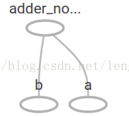
7：一个计算图可以参数化的接收外部的输入，作为一个 placeholders(占位符)，一个占位符是 允许后面提供一个值的。

   
   
a = tf.placeholder(tf.float32)
b = tf.placeholder(tf.float32)
adder_node = a + b # + provides a shortcut for tf.add(a, b)
   
   

这里有点像一个function (函数)或者lambda表达式，我们定义了2个输入参数a和b，然后提供一个在它们之上的操作。我们可以使用

feed_dict(传递字典)参数传递具体的值到run方法的占位符来进行多个输入，从而来计算这个图。

   
   
print(sess.run(adder_node, {a: 3, b: 4.5}))
print(sess.run(adder_node, {a: [ 1, 3], b: [ 2, 4]}))
   
   

结果是：

   
   
7.5
[ 3. 7.]
   
   

在TensorBoard，计算图类似于这样：

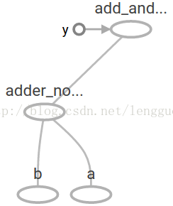
8：我们可以增加另外的操作来让计算图更加复杂，比如

   
   
add_and_triple = adder_node * 3.
print(sess.run(add_and_triple, {a: 3, b: 4.5}))
输出结果是：
22.5
   
   

在TensorBoard，计算图类似于这样：

9：在机器学习中，我们通常想让一个模型可以接收任意多个输入，比如大于1个，好让这个模型 可以被训练，在不改变输入的情况下,

我们需要改变这 个计算图去获得一个新的输出。变量允许 我们增加可训练的参数到这个计算图中，它们被构造成有一个类型和初始值：

   
   
W = tf.Variable([ .3], dtype=tf.float32)
b = tf.Variable([ -.3], dtype=tf.float32)
x = tf.placeholder(tf.float32)
linear_model = W*x + b
   
   

10 ：当你调用 tf.constant 时 常量被初始化， 它们的值是不可以改变的 ，而变量当你调用 tf.Variable 时没有被初始化，

在TensorFlow程序中要想初始化这 些变量，你必须明确调用一个特定的操作， 如下：

   
   
init = tf.global_variables_initializer()
sess.run(init)
   
   

11：要实现初始化所有全局变量的TensorFlow子图的的处理是很重要的，直到我们调用 sess.run， 这些变量都是未被初始化的。

既然x是一个占位符， 我们就可以同时地对多个x的值进行求值 linear_model ，例如：

   
   
print(sess.run(linear_model, {x: [ 1, 2, 3, 4]}))
求值linear_model
输出为
[ 0. 0.30000001 0.60000002 0.90000004]
   
   

12 ：我们已经创建了一个模型，但是我们至今不知道它是多好，在这些训练数据上对这个模型进行评估，我们需要一个

y占位符来提供一个期望的值， 并且我们需要写一个 loss function (损失 函数)，一个损失函数度量当前的模型和提供

的数据有多远，我们将会使用一个标准的损失模式 来线性回 归，它的增量平方和就是当前模型与提供的数据之间的损失

， linear_model - y 创建一 个向量，其中每个元素都是对应的示例错误增量。这个错误 的方差我们称为 tf.square 。然后

，我 们合计所有的错误方差用以创建一个标量，用 tf.reduce_sum 抽象出所有示例的错误。

   
   
y = tf.placeholder(tf.float32)
squared_deltas = tf.square(linear_model - y)
loss = tf.reduce_sum(squared_deltas)
print(sess.run(loss, {x: [ 1, 2, 3, 4], y: [ 0, -1, -2, -3]}))
输出的结果为
23.66
   
   

13：我们分配一个值给W和b(得到一个完美的值是-1和1)来手动改进这一点,一个变量被初始化一个值 会调用 tf.Variable ，

但是可以用tf.assign来改变这 个值，例如： fixW = tf.assign(W, [- 1. ])

   
   
fixb = tf.assign(b, [ 1.])
sess.run([fixW, fixb])
print(sess.run(loss, {x: [ 1, 2, 3, 4], y: [ 0, -1, -2, -3]}))
最终打印的结果是：
0.0
   
   

14 ： tf.train API TessorFlow提供 optimizers (优化器)，它能慢慢改变每一个变量以最小化 损 失 函 数，最简单的优化器是

gradient descent (梯度 下降)，它根据变量派生出损失的大小, 来修改每个变量。通常手工计算变量符号是乏味且容易出错的，

因此，TensorFlow使用函数 tf.gradients 给 这个模型一个描述，从而能自动地提供衍生品，简而言之，优化器通常会为你做 这个。例如：

   
   
optimizer = tf.train.GradientDescentOptimizer( 0.01)
train = optimizer.minimize(loss)
sess.run(init) # reset values to incorrect defaults.
for iin range( 1000):
sess.run(train, {x: [ 1, 2, 3, 4], y: [ 0, -1, -2, -3]})

print(sess.run([W, b]))
输出结果为
[array([ -0.9999969], dtype=float32), array([ 0.99999082], dtype=float32)]
   
   

现在你已经完成了实际的机器学习，尽管这个简单的线性回归模型不要求太多TensorFlow core 代码， 更复杂的模型和

方法将数据输入到模型中， 需要跟多的代码，因此TensorFlow为常见模式 ，结构和功能提供更高级别的抽象，我们将会

在下一个章节学习这些抽象。

15 ： tf.estimator tf.setimator 是一个更高级别的TensorFlow库，它简化了机械式的机器 学习，包含以下几个方面：

• running training loops 运行训练循环
• running evaluation loops 运行求值循环
• managing data sets 管理数据集合

tf.setimator 定义了很多相同的模型。

16： A custom model tf.setimator 没有把你限制在预定好的模型中，假设我们想要创建一个自 定义的模型，它不是由

TensorFlow建成的。我还是能 保持这些数据集合，输送，训练高级别的 抽象；例如：tf.estimator;

17：现在你有了关于TensorFlow的一个基本工作知识，我们还有更多教程，它能让你学习更多。如果你是一 个机器学习初学者，

你可以继续 学习 MNIST for beginners ， 否则你可以学习 Deep MNIST for experts .

完整的代码：

   
   
import tensorflow as tf
node1 = tf.constant( 3.0, dtype=tf.float32)
node2 = tf.constant( 4.0) # also tf.float32 implicitly
print(node1, node2)

sess = tf.Session()
print(sess.run([node1, node2]))

# from __future__ import print_function
node3 = tf.add(node1, node2)
print( "node3:", node3)
print( "sess.run(node3):", sess.run(node3))


# 占位符
a = tf.placeholder(tf.float32)
b = tf.placeholder(tf.float32)
adder_node = a + b # + provides a shortcut for tf.add(a, b)

print(sess.run(adder_node, {a: 3, b: 4.5}))
print(sess.run(adder_node, {a: [ 1, 3], b: [ 2, 4]}))

add_and_triple = adder_node * 3.
print(sess.run(add_and_triple, {a: 3, b: 4.5}))


# 多个变量求值
W = tf.Variable([ .3], dtype=tf.float32)
b = tf.Variable([ -.3], dtype=tf.float32)
x = tf.placeholder(tf.float32)
linear_model = W*x + b

# 变量初始化
init = tf.global_variables_initializer()
sess.run(init)

print(sess.run(linear_model, {x: [ 1, 2, 3, 4]}))

# loss function
y = tf.placeholder(tf.float32)
squared_deltas = tf.square(linear_model - y)
loss = tf.reduce_sum(squared_deltas)
print( "loss function", sess.run(loss, {x: [ 1, 2, 3, 4], y: [ 0, -1, -2, -3]}))

ss = ( 0 -0)*( 0 -0) + ( 0.3+ 1)*( 0.3+ 1) + ( 0.6+ 2)*( 0.6+ 2) + ( 0.9+ 3)*( 0.9+ 3) # 真实算法
print( "真实算法ss", ss)

print(sess.run(loss, {x: [ 1, 2, 3, 4], y: [ 0, 0.3, 0.6, 0.9]})) # 测试参数

# ft.assign 变量重新赋值
fixW = tf.assign(W, [ -1.])
fixb = tf.assign(b, [ 1.])
sess.run([fixW, fixb])
print(sess.run(linear_model, {x: [ 1, 2, 3, 4]}))
print(sess.run(loss, {x: [ 1, 2, 3, 4], y: [ 0, -1, -2, -3]}))


# tf.train API
optimizer = tf.train.GradientDescentOptimizer( 0.01) # 梯度下降优化器
train = optimizer.minimize(loss) # 最小化损失函数
sess.run(init) # reset values to incorrect defaults.
for i in range( 1000):
sess.run(train, {x: [ 1, 2, 3, 4], y: [ 0, -1, -2, -3]})

print(sess.run([W, b]))


print( "------------------------------------1")

# Complete program:The completed trainable linear regression model is shown here:完整的训练线性回归模型代码
# Model parameters
W = tf.Variable([ .3], dtype=tf.float32)
b = tf.Variable([ -.3], dtype=tf.float32)
# Model input and output
x = tf.placeholder(tf.float32)
linear_model = W*x + b
y = tf.placeholder(tf.float32)

# loss
loss = tf.reduce_sum(tf.square(linear_model - y)) # sum of the squares
# optimizer
optimizer = tf.train.GradientDescentOptimizer( 0.01)
train = optimizer.minimize(loss)

# training data
x_train = [ 1, 2, 3, 4]
y_train = [ 0, -1, -2, -3]
# training loop
init = tf.global_variables_initializer()
sess = tf.Session()
sess.run(init) # reset values to wrong
for i in range( 1000):
sess.run(train, {x: x_train, y: y_train})

# evaluate training accuracy
curr_W, curr_b, curr_loss = sess.run([W, b, loss], {x: x_train, y: y_train})
print( "W: %s b: %s loss: %s"%(curr_W, curr_b, curr_loss))


print( "------------------------------------2")

# tf.estimator 使用tf.estimator实现上述训练
# Notice how much simpler the linear regression program becomes with tf.estimator:
# NumPy is often used to load, manipulate and preprocess data.
import numpy as np
import tensorflow as tf

# Declare list of features. We only have one numeric feature. There are many
# other types of columns that are more complicated and useful.
feature_columns = [tf.feature_column.numeric_column( "x", shape=[ 1])]

# An estimator is the front end to invoke training (fitting) and evaluation
# (inference). There are many predefined types like linear regression,
# linear classification, and many neural network classifiers and regressors.
# The following code provides an estimator that does linear regression.
estimator = tf.estimator.LinearRegressor(feature_columns=feature_columns)

# TensorFlow provides many helper methods to read and set up data sets.
# Here we use two data sets: one for training and one for evaluation
# We have to tell the function how many batches
# of data (num_epochs) we want and how big each batch should be.
x_train = np.array([ 1., 2., 3., 4.])
y_train = np.array([ 0., -1., -2., -3.])
x_eval = np.array([ 2., 5., 8., 1.])
y_eval = np.array([ -1.01, -4.1, -7, 0.])
input_fn = tf.estimator.inputs.numpy_input_fn(
{ "x": x_train}, y_train, batch_size= 4, num_epochs= None, shuffle= True)
train_input_fn = tf.estimator.inputs.numpy_input_fn(
{ "x": x_train}, y_train, batch_size= 4, num_epochs= 1000, shuffle= False)
eval_input_fn = tf.estimator.inputs.numpy_input_fn(
{ "x": x_eval}, y_eval, batch_size= 4, num_epochs= 1000, shuffle= False)

# We can invoke 1000 training steps by invoking the method and passing the
# training data set.
estimator.train(input_fn=input_fn, steps= 1000)

# Here we evaluate how well our model did.
train_metrics = estimator.evaluate(input_fn=train_input_fn)
eval_metrics = estimator.evaluate(input_fn=eval_input_fn)
print( "train metrics: %r"% train_metrics)
print( "eval metrics: %r"% eval_metrics)


print( "------------------------------------3")

# A custom model：客户自定义实现训练
# Declare list of features, we only have one real-valued feature
def model_fn(features, labels, mode):
# Build a linear model and predict values
W = tf.get_variable( "W", [ 1], dtype=tf.float64)
b = tf.get_variable( "b", [ 1], dtype=tf.float64)
y = W*features[ 'x'] + b
# Loss sub-graph
loss = tf.reduce_sum(tf.square(y - labels))
# Training sub-graph
global_step = tf.train.get_global_step()
optimizer = tf.train.GradientDescentOptimizer( 0.01)
train = tf.group(optimizer.minimize(loss),
tf.assign_add(global_step, 1))
# EstimatorSpec connects subgraphs we built to the
# appropriate functionality.
return tf.estimator.EstimatorSpec(
mode=mode,
predictions=y,
loss=loss,
train_op=train)

estimator = tf.estimator.Estimator(model_fn=model_fn)
# define our data sets
x_train = np.array([ 1., 2., 3., 4.])
y_train = np.array([ 0., -1., -2., -3.])
x_eval = np.array([ 2., 5., 8., 1.])
y_eval = np.array([ -1.01, -4.1, -7., 0.])
input_fn = tf.estimator.inputs.numpy_input_fn(
{ "x": x_train}, y_train, batch_size= 4, num_epochs= None, shuffle= True)
train_input_fn = tf.estimator.inputs.numpy_input_fn(
{ "x": x_train}, y_train, batch_size= 4, num_epochs= 1000, shuffle= False)
eval_input_fn = tf.estimator.inputs.numpy_input_fn(
{ "x": x_eval}, y_eval, batch_size= 4, num_epochs= 1000, shuffle= False)

# train
estimator.train(input_fn=input_fn, steps= 1000)
# Here we evaluate how well our model did.
train_metrics = estimator.evaluate(input_fn=train_input_fn)
eval_metrics = estimator.evaluate(input_fn=eval_input_fn)
print( "train metrics: %r"% train_metrics)
print( "eval metrics: %r"% eval_metrics)