Tensorflow卷积网络实现对CIFAR图像的分类

版权声明：本文为博主原创文章，遵循 CC 4.0 BY-SA 版权协议，转载请附上原文出处链接和本声明。

本文链接： https://blog.csdn.net/weixin_44547562/article/details/102734492

CIFAR数据集简介

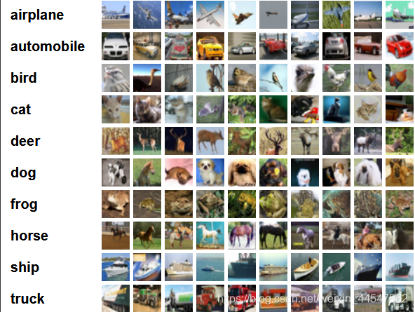
该数据集共有60000张彩色图像，这些图像是32*32，分为10个类，每类6000张图。这里面有50000张用于训练，构成了5个训练批，每一批10000张图；另外10000用于测试，单独构成一批。测试批的数据里，取自10类中的每一类，每一类随机取1000张。抽剩下的就随机排列组成了训练批。注意一个训练批中的各类图像并不一定数量相同，总的来看训练批，每一类都有5000张图。

下面这幅图就是列举了10各类，每一类展示了随机的10张图片：

下载数据集

import urllib.request
import os
import tarfile
import tensorflow as tf

# 创建文件夹
filepath = 'data/'
if not os.path.exists(filepath):
    os.mkdir(filepath)
    print('创建成功')
else:
    print("文件夹已存在")
    
# 下载数据文件
url = 'https://www.cs.toronto.edu/~kriz/cifar-10-python.tar.gz'
filepath = 'data/cifar-10-python.tar.gz'
if not os.path.isfile(filepath):
    result = urllib.request.urlretrieve(url, filepath)
    print('downlanded: ',result)
else:
    print('Data file already exists')
    
# 解压数据文件
if not os.path.exists("data/cifar-10-batches-py"):
    tflie = tarfile.open("data/cifar-10-python.tar.gz","r:gz")
    result = tflie.extractall('data/')
    print('Extracted to ./data/cifar-10-batches-py')
    print('Finished it')
else:
    print('Directory already exists')

导入数据集

import os
import numpy as np
import pickle as p

def load_CIFAR_batch(filename):
    with open(filename,'rb')as f:
        data_dict = p.load(f, encoding='bytes')
        images = data_dict[b'data']
        labels = data_dict[b'labels']

        # 把原始数据结构调整为：BCWH
        images = images.reshape(10000,3,32,32)
        # tensorflow处理图像数据的结构：BWHC
        # 把通道数据C移动到最后一个维度
        images = images.transpose(0,2,3,1)

        labels = np.array(labels)

        return images,labels

def load_CIFAR_data(data_dir):
    images_train = []
    labels_train = []
    for i in range(5):
        f = os.path.join(data_dir,'data_batch_%d'%(i+1))
        print('loading ',f)
        # 调用load_CIFAR_batch()获得批量的图像及其对应的标签
        image_batch,label_batch = load_CIFAR_batch(f)
        images_train.append(image_batch)
        labels_train.append(label_batch)
        Xtrain = np.concatenate(images_train)
        Ytrain = np.concatenate(labels_train)
        del image_batch,label_batch
        
    Xtest,Ytest = load_CIFAR_batch(os.path.join(data_dir,'test_batch'))
    print('finish loadding CIFAR-10 data')
    
    # 返回训练集的图像和标签，测试集的图像和标签
    return Xtrain,Ytrain,Xtest,Ytest

data_dir = 'data/cifar-10-batches-py'
Xtrain,Ytrain,Xtest,Ytest = load_CIFAR_data(data_dir)

显示数据集信息

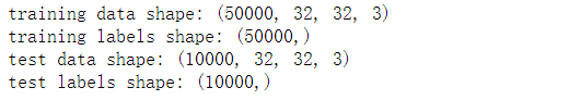
print('training data shape:',Xtrain.shape)
print('training labels shape:',Ytrain.shape)
print('test data shape:',Xtest.shape)
print('test labels shape:',Ytest.shape)

得到如下结果：

数据预处理

图像数据预处理

# 查看图像数据信息
# 显示第一个图的第一个像素点
print(Xtrain[0][0][0])

# 归一化
Xtrain_normalize = Xtrain.astype('float32')/255.0
Xtest_normalize = Xtest.astype('float32')/255.0
print(Xtrain_normalize[0][0][0])

标签数据预处理——独热编码

from sklearn.preprocessing import OneHotEncoder

encoder = OneHotEncoder(sparse=False,categories='auto')

yy = [[0],[1],[2],[3],[4],[5],[6],[7],[8],[9]]
encoder.fit(yy)
# 转置
Ytrain_reshpe = Ytrain.reshape(-1,1)
Ytest_reshpe = Ytest.reshape(-1,1)
# 独热编码
Ytrain_onehot = encoder.transform(Ytrain_reshpe)
Ytest_onehot = encoder.transform(Ytest_reshpe)

定义共享参数

# 定义权值
def weight(shape):
    return tf.Variable(tf.truncated_normal(shape,stddev=0.1),name='W')

# 定义偏置项
def bias(shape):
    return tf.Variable(tf.constant(0.1,shape=shape),name='b')

# 定义卷积操作
# 步长为1，paddding为'SAME'，即卷积后图片大小不变化
def conv2d(x,W):
    return tf.nn.conv2d(x,W,strides=[1,1,1,1],padding='SAME')

# 定义池化操作
# 步长为2，即原尺寸的长和宽除以2
def max_pool(x):
    return tf.nn.max_pool(x,ksize=[1,2,2,1],strides=[1,2,2,1],padding='SAME')

定义网络结构

# 输入层
# 32x32图像，通道为3(RGB)
# 用tf.name_scope('inputt_layer')将下面结构打包成input_layer
with tf.name_scope('inputt_layer'):
    x = tf.placeholder('float',shape=[None,32,32,3],name='X')
    
# 第一个卷积层
# 输入通道：3，输出通道：32，卷积后图像尺寸不变，依然是32x32
with tf.name_scope('conv_1'):
    W1 = weight([3,3,3,32]) # [k_wight,k_height,input_chn,output_chn]
    b1 = bias([32]) # 与output_chn一致
    conv_1 = tf.nn.relu(conv2d(x,W1)+b1)
    
# 第一个池化层
# 将32x32的图像缩小为16x16，不改变通道数
with tf.name_scope('pool_1'):
    pool_1 = max_pool(conv_1)
    
# 第二个卷积层
# 输入通道：32，输出通道：64，卷积后图像尺寸不变，依然是32x32
with tf.name_scope('conv_2'):
    W2 = weight([3,3,32,64]) # [k_wight,k_height,input_chn,output_chn]
    b2 = bias([64]) # 与output_chn一致
    conv_2 = tf.nn.relu(conv2d(pool_1,W2)+b2)

# 第二个池化层
# 将16x16的图像缩小为8x8，不改变通道数
with tf.name_scope('pool_2'):
    pool_2 = max_pool(conv_2)
    
# 全连接层
# 将64个8x8的图像转换为一维的向量，长度是64*8*8=4096
# 158个神经元
with tf.name_scope('fc'):
    W3 = weight([4096,158])
    b3 = bias([158])
    flat = tf.reshape(pool_2,[-1,4096])# 将pool_2展开为1行4096列的向量
    h = tf.nn.relu(tf.matmul(flat,W3)+b3)
    # 使用dropout方法使20%的神经元消失，防止神经网络过拟合
    h_dropout = tf.nn.dropout(h,keep_prob=0.8)
    
# 输出层
# 输出层有10个神经元，对应10个类别
with tf.name_scope('output_layer'):
    W4 = weight([158,10])
    b4 = bias([10])
    pred = tf.nn.softmax(tf.matmul(h_dropout,W4)+b4)

构建模型

with tf.name_scope('optimizer'):
    # 定义占位符
    y = tf.placeholder('float',shape=[None,10],name='label')
    # 定义损失函数
    loss_fun = tf.reduce_mean(
        tf.nn.softmax_cross_entropy_with_logits
        (logits=pred,labels=y))
    # 选择优化器
    lr = 0.0001
    opt = tf.train.AdamOptimizer(lr).minimize(loss_fun)

定义准确率

with tf.name_scope('evaluation'):
    # tf.argmax(x,1)返回x中每一行最大值的位置
    correct_prediction = tf.equal(tf.argmax(pred,1),tf.argmax(y,1))
    accuracy = tf.reduce_mean(tf.cast(correct_prediction,'float'))

其中tf.argmax(x,1)返回x中每一行最大值的位置。

定义返回下一个epoch的函数

def next_epoch(num, batch_size):
    index = np.random.randint(0,num-1,batch_size)
    batch_x = Xtrain_normalize[index]
    batch_y = Ytrain_onehot[index]
    return batch_x,batch_y

训练模型

import os
from time import time

train_epochs = 50
batch_size = 50
total_batch = int(len(Xtrain)/batch_size)
display_step = 1
epoch_list = []
accuracy_list = []
loss_list = []

# epoch = tf.Variable(0,name='epoch',trainable=False)

startTime = time()

init = tf.global_variables_initializer()
with tf.Session() as sess:
    sess.run(init)
    for epoch in range(train_epochs):
        for i in range(total_batch):
            batch_x, batch_y = next_epoch(50000,batch_size)
            sess.run(opt,feed_dict={x:batch_x,y:batch_y})
            
        loss,acc = sess.run([loss_fun,accuracy],feed_dict={x:batch_x,y:batch_y})
        if epoch%display_step == 0:
                    print("Train Epoch:%02d" % (epoch+1),"Loss=%f" % loss, "Accuracy=%.4f" % acc)
        epoch_list.append(ep+1)
        loss_list.append(loss)
        accuracy_list.append(acc)
    
time_cost = time() - startTime
print("Train finished takes:%.4f" % time_cost)

损失（准确率）可视化

%matplotlib inline
import matplotlib.pyplot as plt

fig = plt.gcf()
fig.set_size_inches(4,2)
plt.plot(loss_list,label='loss')
plt.ylabel('loss')
plt.xlabel('epoch')
plt.title('Loss')
plt.legend(['loss'],loc='upper right')