本文是数据可视化的第二篇练习文,目的是承接上一篇中国(2002-2018)全国各省结婚率和离婚率数据可视化
该篇文章主要使用的是Python数据可视化,用来分析北京地区从2002到2018年房价的趋势变化
为了方便读者理解,在写的篇幅中,不加入代码,所有代码放在最后的附录里。
一:加载数据以及相应的库包

二:检验数据
加载成功后,需要验证数据的正确性

三:数据处理
对于数据的处理,我们一般查看数据中的缺失值

以上6列数据具有缺失值。
然后我们计算数据中空列缺失值的个数
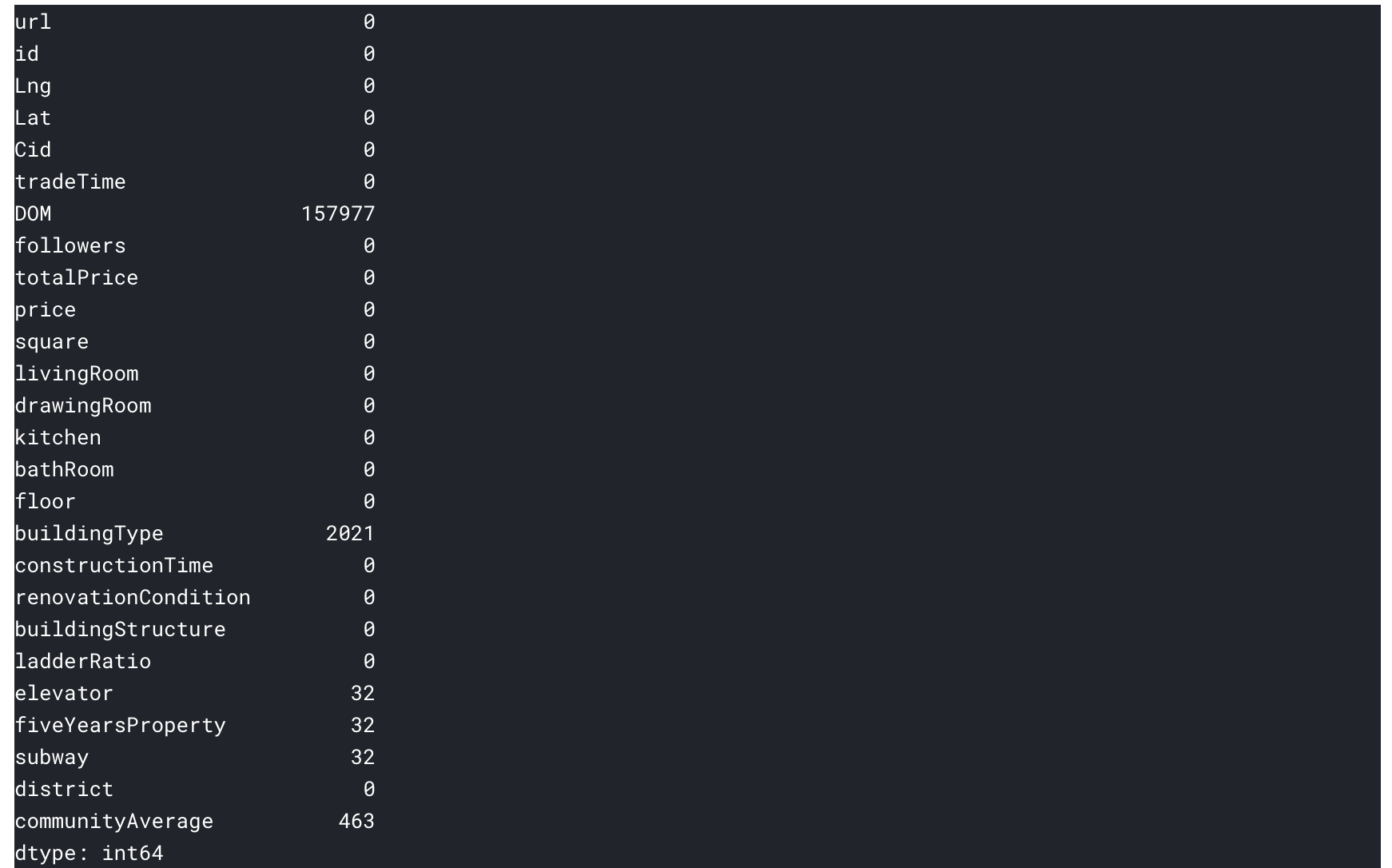
另外解释一下数据中各列值的含义
url: the url which fetches the data
id: the id of transaction
lng: 经
lat: 纬
cid: community id
tradeTime: the time of transaction
followers: the number of people follow the transaction.
price: the average price by square
square: the square of house(1m*1m)
livingRoom: the number of living room
drawingRoom: the number of drawing room
kitchen: the number of kitchen
bathroom: the number of bathroom
constructionTime: 建造年代
floor: the height of the house. I will turn the Chinese characters to English in the next version.
buildingType: including tower( 1 ) , bungalow( 2 ),combination of plate and tower( 3 ), plate( 4 ).
renovationCondition: including other( 1 ), rough( 2 ),Simplicity( 3 ), hardcover( 4 )
buildingStructure: including unknow( 1 ), mixed( 2 ), brick and wood( 3 ), brick and concrete( 4 ),steel( 5 ) and steel-concrete composite ( 6 ).
ladderRatio: the proportion between number of residents on the same floor and number of elevator of ladder. It describes how many ladders a resident have on average.
elevator: have ( 1 ) or not have elevator( 0 )
fiveYearsProperty: if the owner have the property for less than 5 years,
district列表中各区指代内容:
1:东城区
2:丰台区
3:亦庄
4:大兴区
5:房山
6:昌平区
7:朝阳区
8.海淀区
9.石景山
10:西城区
11:通州区
12门头沟
13:顺义区
查看各值的数量:

若空列数量占总过多或者不影响关键信息,可以直接删除空列
其中,
axis=1 删除 columns
axis=0 删除 rows
四、数据可视化
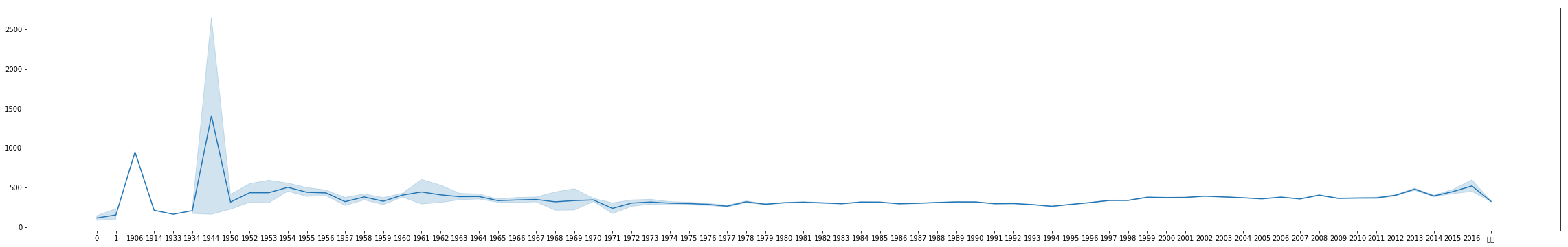
- 北京(2002-2018)年房价总体走势图(单价)
元/平方米

- 北京房子总价与房屋面积之间的关系:

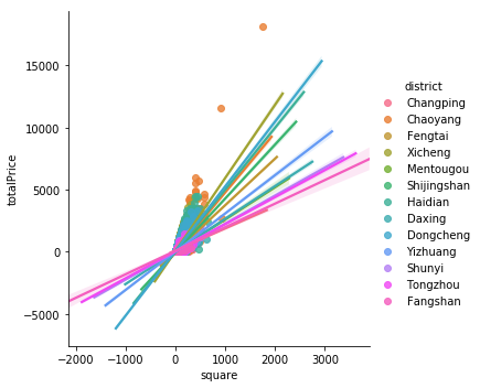
- 北京各区房子总价与房屋面积之间的关系
- 北京各区房价单价的中位数(元/平方米)
可以看到西城最高,东城次之

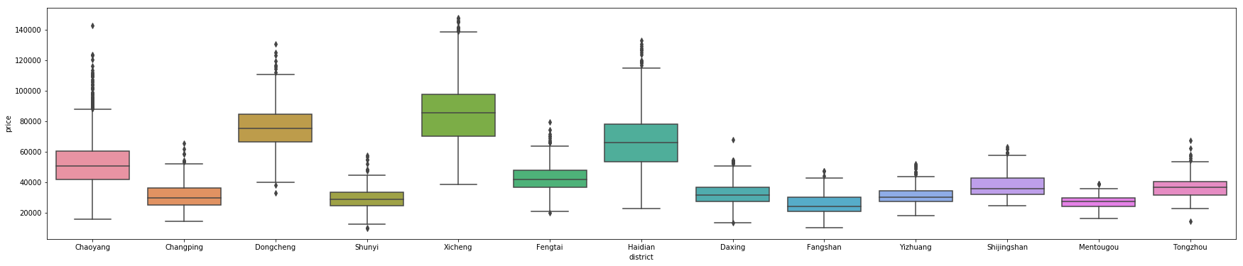
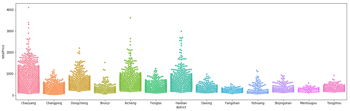
- 区域与房子单价之间的关系图(盒图)
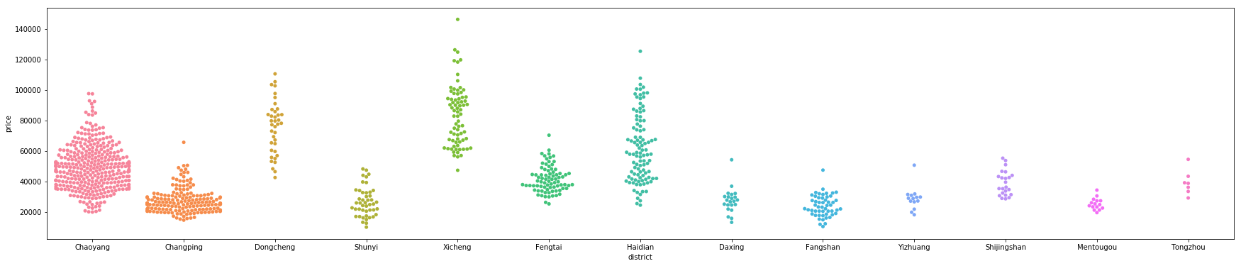
- 区域与房子单价之间的关系图(分类散点图)
- 各区房价与总价之间的关系
可以明显看到,朝阳区3千万以上好在比其它区多,西城次之,富人应该多集居在朝阳,西城,海淀
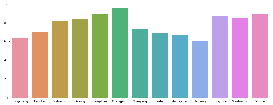
- 北京各区房价的中位数
中位数代表着普通百姓的消费能力,可以看到,西城,东城,海淀最高

- 北京各区房子面积分布
朝阳,昌平的大房比较多

- 各区房子面积的中位数
昌平居冠,西城最小
五、买房应该注意什么
1.人们喜欢什么价位的房子
可以发现1000万以下的房子followers比较多,说明这个段位以下的房子面向的人群最广

2.地铁对房价的影响
可以很明显的发现,各区周围有地铁的房子,比无地铁的房子,单价要高几千,其中海淀,门口沟,朝阳,房山影响很明显,说明这几个区居住的上班族多

3.建造年代与房子单价的关系(单位:万/平方米)
最近几年的房子以及老房普遍比新房贵,可能是区域的关系,因为老房多位于老城区,房价比较高

4.建造年代与房子总价的关系(单位:百万/套)
5.人们更喜欢什么楼层的房子
可以看到5楼和6楼比较抢手

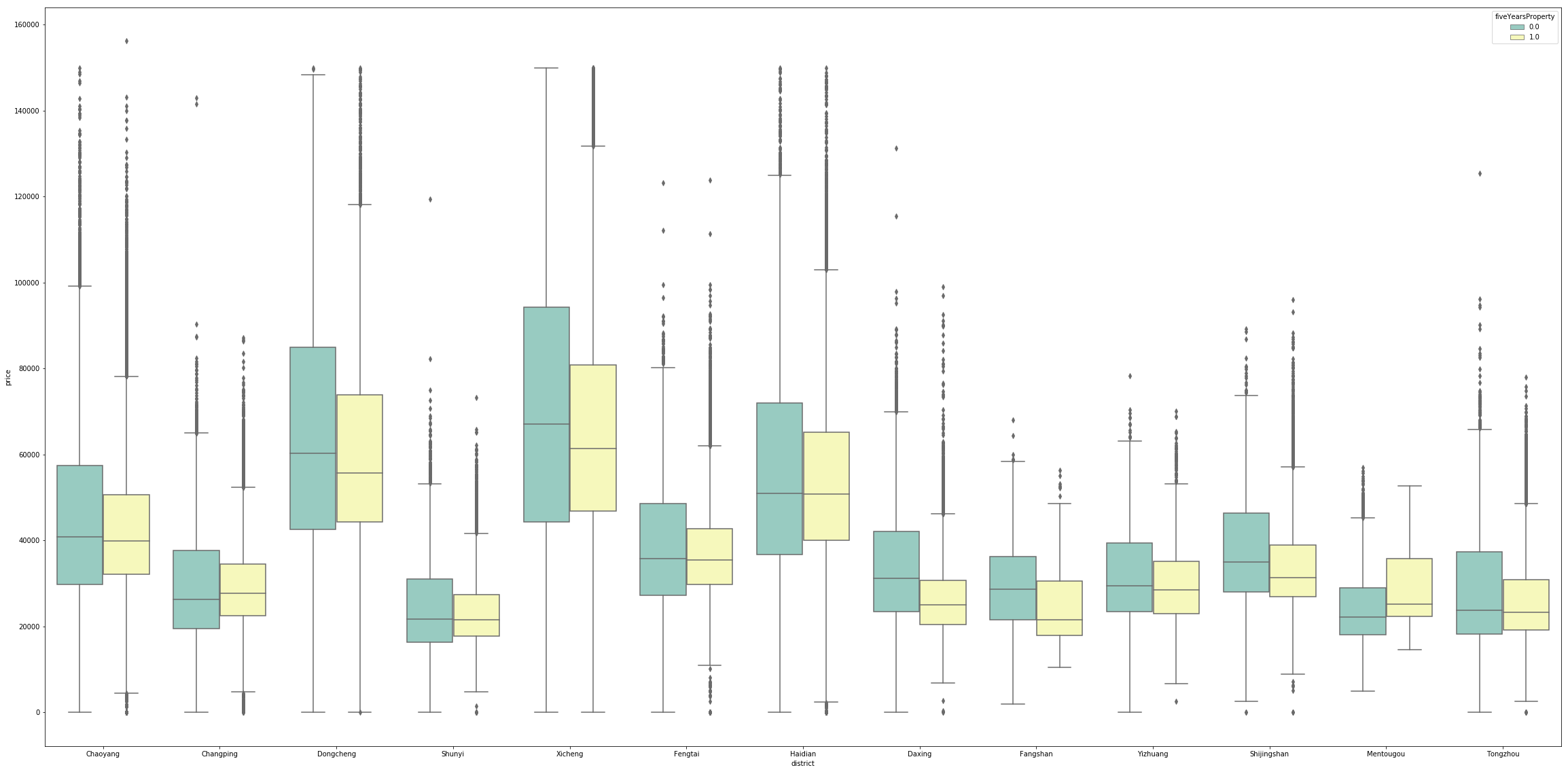
6.五年产权对房价的影响
可以看到政策的影线,没有到五年产权的房子单价普遍贵一些
六、总结
以上是使用Python对北京房价的数据可视化,可以发现一些有趣的信息。笔者准备使用热力图显示相应的信息,但是由于地图测绘法的关系,echarts.js的北京地图信息不能使用了,如果有谁知道其它工具的化可以给我留言,期望改进,比心!
附录
本文所有的代码:
# This Python 3 environment comes with many helpful analytics libraries installed
# It is defined by the kaggle/python docker image: https://github.com/kaggle/docker-python
# For example, here's several helpful packages to load in
import numpy as np # linear algebra
import pandas as pd # data processing, CSV file I/O (e.g. pd.read_csv)
# Input data files are available in the "../input/" directory.
# For example, running this (by clicking run or pressing Shift+Enter) will list all files under the input directory
import os
for dirname, _, filenames in os.walk('/kaggle/input'):
for filename in filenames:
print(os.path.join(dirname, filename))
# Any results you write to the current directory are saved as output.
import matplotlib.pyplot as plt
%matplotlib inline
import seaborn as sns
file_path = "../input/lianjia/new.csv"
file_content = pd.read_csv(file_path,encoding='gbk')
file_temporary = pd.read_csv(file_path,encoding='gbk',index_col='tradeTime',parse_dates=True)
file_temporary.sort_index()
df2=pd.DataFrame(file_temporary.sort_index())
plt.figure(figsize=(30,6))
sns.lineplot(data=df2['price'],label='the trend of housing price in beijing')
df = pd.DataFrame(file_content)
with_missing_value = [col for col in df.columns if df[col].isnull().any()]
count_missing_null_column = (df.isnull().sum())
df = df.drop(with_missing_value,axis=1)
df['price'].shape
sns.regplot(x=df.loc[0:10000,'square'],y=df.loc[0:10000,'totalPrice'])
df_copy= df.copy()
df_copy.district[df.district==1]='Dongcheng'
df_copy.district[df.district==2]='Fengtai'
df_copy.district[df.district==3]='Yizhuang'
df_copy.district[df.district==4]='Daxing'
df_copy.district[df.district==5]='Fangshan'
df_copy.district[df.district==6]='Changping'
df_copy.district[df.district==7]='Chaoyang'
df_copy.district[df.district==8]='Haidian'
df_copy.district[df.district==9]='Shijingshan'
df_copy.district[df.district==10]='Xicheng'
df_copy.district[df.district==11]='Tongzhou'
df_copy.district[df.district==12]='Mentougou'
df_copy.district[df.district==13]='Shunyi'
sns.lmplot(x="square", y="totalPrice", hue="district", data=df_copy)
plt.figure(figsize=(30,6))
sns.swarmplot(x=df_copy.loc[0:10000,'district'],
y=df_copy.loc[0:10000,'price'])
plt.figure(figsize=(30,6))
sns.boxplot(x=df_copy.loc[0:10000,'district'], y=df_copy.loc[0:10000,'price'])
len=[]
for i in range(1,14):
len.append(df.price[df.district==i].median())
print (len)
plt.figure(figsize=(16,6))
sns.barplot(x=['Dongcheng','Fengtai','Yizhuang','Daxing','Fangshan','Changping',
'Chaoyang','Haidian','Shijingshan','Xicheng','Tongzhou','Mentougou'
,'Shunyi'
],y=len)
plt.figure(figsize=(20,6))
sns.swarmplot(x=df_copy.loc[0:10000,'district'],
y=df_copy.loc[0:10000,'totalPrice'])
total_len=[]
for i in range(1,14):
total_len.append(df.totalPrice[df.district==i].median())
print (total_len)
plt.figure(figsize=(16,6))
sns.barplot(x=['Dongcheng','Fengtai','Yizhuang','Daxing','Fangshan','Changping',
'Chaoyang','Haidian','Shijingshan','Xicheng','Tongzhou','Mentougou'
,'Shunyi'
],y=total_len)
plt.figure(figsize=(20,6))
sns.swarmplot(x=df_copy.loc[0:10000,'district'],
y=df_copy.loc[0:10000,'square'])
plt.figure(figsize=(20,6))
sns.boxplot(x=df_copy.loc[0:10000,'district'],
y=df_copy.loc[0:10000,'square'])
total_square=[]
for i in range(1,14):
total_square.append(df.square[df.district==i].median())
print (total_len)
plt.figure(figsize=(16,6))
sns.barplot(x=['Dongcheng','Fengtai','Yizhuang','Daxing','Fangshan','Changping',
'Chaoyang','Haidian','Shijingshan','Xicheng','Tongzhou','Mentougou'
,'Shunyi'
],y=total_square)
plt.figure(figsize=(20,6))
sns.regplot(x=df.loc[0:10000,'followers'],y=df.loc[0:10000,'totalPrice'])
pd_construct_time = pd.read_csv(file_path,encoding='gbk',index_col='constructionTime',parse_dates=True)
df_construct = pd.DataFrame(pd_construct_time)
plt.figure(figsize=(40,6))
sns.lineplot(data=df_construct["price"])
plt.figure(figsize=(40,6))
sns.lineplot(data=df_construct["totalPrice"])
plt.figure(figsize=(40,6))
sns.boxplot(x="constructionTime", y="totalPrice", data=df)
plt.figure(figsize=(40,20))
ax = sns.boxplot(x="district", y="price", hue="subway",data=df_copy, palette="Set3")
plt.figure(figsize=(40,20))
ax = sns.boxplot(x="district", y="price", hue="fiveYearsProperty",data=df_copy, palette="Set3")
plt.figure(figsize=(70,20))
ax = sns.boxplot(x="district", y="price", hue="buildingStructure",data=df, palette="Set3")
plt.figure(figsize=(50,6))
sns.boxplot(x=df.loc[0:10000,'floor'],y=df.loc[0:10000,'followers'])
first=[]
second=[]
for i,j in zip(df.floor,df.followers):
temp=i.split(" ")
if len(temp)==2:
first.append(temp[1])
second.append(j)
output = pd.DataFrame({
'floor':first,
'followers':second
})
output.to_csv('floor-followers.csv',index=False)
floor_price = pd.read_csv('floor-followers.csv')
df = pd.DataFrame(floor_price)
df_sorted=df.sort_values(by='floor')
plt.figure(figsize=(30,30))
sns.boxplot(x="floor",y="followers",data=df_sorted)