python机器学习基础教程-监督学习

1. 分类与回归

　　分类:就是根据给定的标签,把新的数据划分到这些标签中的一个

　　回归:就是根据事物一些属性,来判断这个事物的另一个属性在哪个区间范围

　　　　比如:根据一个人的受教育程度,年龄等,判断这个人的收入在哪个范围内

　　区别: 分类的输出是固定的,离散的,是一个点; 回归的输出是连续的,是区间.

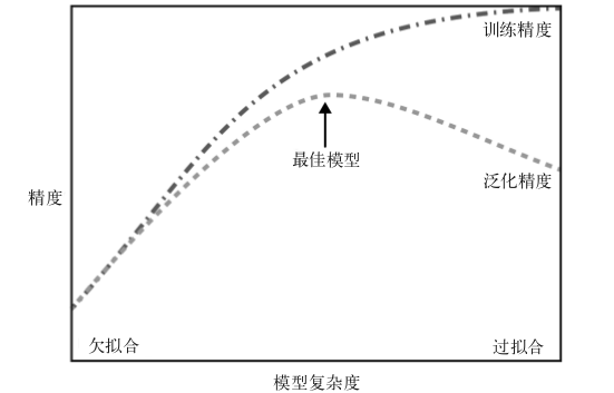
2.泛化,过拟合与欠拟合

　　泛化:一个模型能够对没见过的数据做出准确预测,就说模型能够从训练集泛化到测试集

　　过拟合:构建的模型对于现有的数据来说过于复杂.即模型过分关注训练集的细节,得到在训练集上表现过好,但不能泛化到新数据上.

　　欠拟合:模型在训练集上的表现就很差,就是欠拟合

3.监督学习算法

3.1 一些样本数据集

scikit-learn中数据集都是Bunch对象,包含了真实数据以及一些数据集信息(类似于字典)

3.1.1 forge数据集

导入必要的包

forge数据集有两个特征

# 生成数据集
X, y = mglearn.datasets.make_forge()　　# X和y是forge返回的两个特征
print("X.shape: {}".format(X.shape))　　# X.shape: (26, 2)

# 数据集绘图
mglearn.discrete_scatter(X[:,0],X[:,1],y)　　# 输入X第0列和第1列作为x轴,将y作为y轴
plt.legend(["Class 0", "Class 1"], loc=4)　　# 设置图像的分类名称
plt.xlabel("First feature")　　 # 设置图像x轴的名称
plt.ylabel("Second feature")　　# 设置图像的y轴的名称

3.1.2 wave数据集

wave数据集只有一个输入特征和一个连续的目标变量(x轴表示特征,y轴表示输出)

X, y = mglearn.datasets.make_wave(n_samples=40)　# 生成40个数据,X.shape是(40,1),y.shape是(40,)
plt.plot(X, y, 'o')　　# 图中的点使用圆点表示
plt.ylim(-3, 3)　　　　#设置y轴的区间显示范围
plt.xlabel("Feature")
plt.ylabel("Target")

3.1.3 cancer数据集

cancer数据集记录了乳腺癌肿瘤的临床测量数据,将每个肿瘤标记为良性和恶性(即只有两个标签)

from sklearn.datasets import load_breast_cancer
cancer = load_breast_cancer()
print(cancer.keys())
>>>dict_keys(['data', 'target', 'target_names', 'DESCR', 'feature_names', 'filename'])

print(cancer.data.shape)
print(cancer.target.shape)
print(cancer.target_names)
print(cancer.feature_names)
>>>(569, 30)
>>>(569,) 
>>>['malignant' 'benign'] 
>>>['mean radius' 'mean texture' 'mean perimeter' 'mean area' 'mean smoothness' 'mean compactness' 'mean concavity' 'mean concave points' 'mean symmetry' 'mean fractal dimension' 'radius error' 'texture error' 'perimeter error' 'area error' 'smoothness error' 'compactness error' 'concavity error' 'concave points error' 'symmetry error' 'fractal dimension error' 'worst radius' 'worst texture' 'worst perimeter' 'worst area' 'worst smoothness' 'worst compactness' 'worst concavity' 'worst concave points' 'worst symmetry' 'worst fractal dimension']

{n: v for n, v in zip(cancer.target_names, np.bincount(cancer.target))}
>>>{'malignant': 212, 'benign': 357}

np.bincount的功能:用于统计每个数字的出现次数

x = np.array([0, 1, 1, 3, 2, 1, 7])
a = np.bincount(x)
>>>array([1, 3, 1, 1, 0, 0, 0, 1])
# 如上例,x的范围就是0-7,bincount生成一个np.max(x)+1的array:a
# 当a要生成第一个数时,此时要生成的数字索引为0,就在x中找0出现了多少次,本例为1次,append进来
# 然后a生成第二个数,此时要生成的数组索引是1,就在x中找1出现了多少次,本例为3
# 依次遍历到7,即x

np.bincount的weights参数

w = np.array([0.3, 0.5, 0.2, 0.7, 1., -0.6])
# 我们可以看到x中最大的数为4，因此bin的数量为5，那么它的索引值为0->4
x = np.array([2, 1, 3, 4, 4, 3])
# 索引0 -> 0
# 索引1 -> w[1] = 0.5
# 索引2 -> w[0] = 0.3
# 索引3 -> w[2] + w[5] = 0.2 - 0.6 = -0.4
# 索引4 -> w[3] + w[4] = 0.7 + 1 = 1.7
np.bincount(x,  weights=w)
# 因此，输出结果为：array([ 0. ,  0.5,  0.3, -0.4,  1.7])

3.1.4 波士顿房价数据集

这个数据集包含506个数据点,每个数据点有13个特征

from sklearn.datasets import load_boston
boston = load_boston()
print(boston.data.shape)
>>>(506, 13)

3.2 k近邻

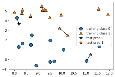
3.2.1 k近邻分类,k-NN算法

取最近的邻居的类别当做自己的类别

mglearn.plots.plot_knn_classification(n_neighbors=1)

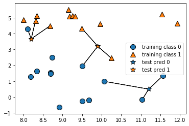
取3个邻居,并根据3个中类别包含最多个数的那个作为自己的类别

mglearn.plots.plot_knn_classification(n_neighbors=3)

3.2.2 应用k近邻算法

导入数据集,并划分训练集和测试集

from sklearn.model_selection import train_test_split
X, y = mglearn.datasets.make_forge()
X_train, X_test, y_train, y_test = train_test_split(X, y, random_state=0)

导入类并实例化knn算法,同时设置参数:邻居的个数

from sklearn.neighbors import KNeighborsClassifier
clf = KNeighborsClassifier(n_neighbors=3)

利用训练集对分类器进行拟合(对于knn就是保存训练集的数据,以便predict的时候计算举例)

clf.fit(X_train, y_train)
>>>KNeighborsClassifier(algorithm='auto', leaf_size=30, metric='minkowski',
                     metric_params=None, n_jobs=None, n_neighbors=3, p=2,
                     weights='uniform')

调用predict方法进行预测

clf.predict(X_test)
>>>array([1, 0, 1, 0, 1, 0, 0])
clf.score(X_test, y_test)
>>>0.8571428571428571

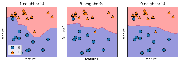
3.2.3 分析KNeighborsClassifier

绘制决策边界: 绘制1个,3个和9个邻居的决策边界

fig, axes = plt.subplots(1, 3, figsize=(10,3))　# 绘制一个1行3列的共3个子图; fig是主图,axes是子图
for n_neighbors, ax in zip([1, 3, 9], axes):
    clf = KNeighborsClassifier(n_neighbors=n_neighbors).fit(X, y)
    mglearn.plots.plot_2d_separator(clf, X, fill=True, eps=0.5, ax=ax, alpha=.4)
    mglearn.discrete_scatter(X[:,0], X[:,1], y, ax=ax)
    ax.set_title("{} neighbor(s)".format(n_neighbors))
    ax.set_xlabel("feature 0")
    ax.set_ylabel("feature 1")
axes[0].legend(loc=3)　　　　# loc标示legend的位置是左下角还是右下角,还是上边

# # # 待更新