卷积神经网络的模型训练技巧

版权声明：本文为博主原创文章，未经博主允许不得转载。 https://blog.csdn.net/cskywit/article/details/88701247

本文cifar10图片分类的例简要说明卷积神经网络中的模型训练技巧，这里我们暂且不提训练的结果的准确度。代码都很简单，不做过多解读。

1.基本的模型

这里使用的就是普通的卷积加池化，最后通过global average pooling输出10个向量经softmax分类：

import tensorflow as tf
import numpy as np
import matplotlib.image as mpimg
import time
import sys
sys.path.append("cifar10_model/")
from cifar10 import *
from cifar10_input import *
data_dir = 'D:/Jupyter_path/TensorflowShiZhan/cifar10_data/cifar-10-binary'
DATA_URL = 'https://www.cs.toronto.edu/~kriz/cifar-10-binary.tar.gz'
batch_size = 128
print("begin")
images_train, labels_train = cifar10_input.inputs(eval_data = False,data_dir = data_dir, batch_size = batch_size)
images_test, labels_test = cifar10_input.inputs(eval_data = True, data_dir = data_dir, batch_size = batch_size)
print("begin data")
def weight_variable(shape):
    initial = tf.truncated_normal(shape, stddev=0.1)
    return tf.Variable(initial)

def bias_variable(shape):
    initial = tf.constant(0.1, shape=shape)
    return tf.Variable(initial)
  
def conv2d(x, W):
    return tf.nn.conv2d(x, W, strides=[1, 1, 1, 1], padding='SAME')

def max_pool_2x2(x):
    return tf.nn.max_pool(x, ksize=[1, 2, 2, 1],
                        strides=[1, 2, 2, 1], padding='SAME')  
                        
def avg_pool_6x6(x):
    return tf.nn.avg_pool(x, ksize=[1, 6, 6, 1],
                        strides=[1, 6, 6, 1], padding='SAME')
# tf Graph Input
x = tf.placeholder(tf.float32, [None, 24,24,3]) # cifar data image of shape 24*24*3
y = tf.placeholder(tf.float32, [None, 10]) # 0-9 数字=> 10 classes


W_conv1 = weight_variable([5, 5, 3, 64])
b_conv1 = bias_variable([64])

x_image = tf.reshape(x, [-1,24,24,3])

h_conv1 = tf.nn.relu(conv2d(x_image, W_conv1) + b_conv1)
h_pool1 = max_pool_2x2(h_conv1)

W_conv2 = weight_variable([5, 5, 64, 64])
b_conv2 = bias_variable([64])

h_conv2 = tf.nn.relu(conv2d(h_pool1, W_conv2) + b_conv2)
h_pool2 = max_pool_2x2(h_conv2)

W_conv3 = weight_variable([5, 5, 64, 10])
b_conv3 = bias_variable([10])
h_conv3 = tf.nn.relu(conv2d(h_pool2, W_conv3) + b_conv3)

nt_hpool3=avg_pool_6x6(h_conv3)#10
nt_hpool3_flat = tf.reshape(nt_hpool3, [-1, 10])
y_conv=tf.nn.softmax(nt_hpool3_flat)

cross_entropy = -tf.reduce_sum(y*tf.log(y_conv))

train_step = tf.train.AdamOptimizer(1e-4).minimize(cross_entropy)

correct_prediction = tf.equal(tf.argmax(y_conv,1), tf.argmax(y,1))
accuracy = tf.reduce_mean(tf.cast(correct_prediction, "float"))
sess = tf.Session()
sess.run(tf.global_variables_initializer())
tf.train.start_queue_runners(sess=sess)
for i in range(15000):#20000
    image_batch, label_batch = sess.run([images_train, labels_train])
    label_b = np.eye(10,dtype=float)[label_batch] #one hot
    train_step.run(feed_dict={x:image_batch, y: label_b},session=sess)
    if i%200 == 0:
        train_accuracy = accuracy.eval(feed_dict={x:image_batch, y: label_b},session=sess)
        print( "step %d, training accuracy %g"%(i, train_accuracy))

2.优化卷积核的方式

在实际训练中，为了加快速度，可以把卷积核分来，如一个3x3的卷积核，可以裁成3x1和1x3两个卷积核，分别对原有输入进行卷积操作，这样可以减少浮点运算中的乘法操作，打打提升运算速度。（数据加载和训练部分代码同上，这里只列出模型设计部分代码）

# tf Graph Input
x = tf.placeholder(tf.float32, [None, 24,24,3]) # cifar data image of shape 24*24*3
y = tf.placeholder(tf.float32, [None, 10]) # 0-9 数字=> 10 classes


W_conv1 = weight_variable([5, 5, 3, 64])
b_conv1 = bias_variable([64])

x_image = tf.reshape(x, [-1,24,24,3])

h_conv1 = tf.nn.relu(conv2d(x_image, W_conv1) + b_conv1)
h_pool1 = max_pool_2x2(h_conv1)
#########################################################new########
W_conv21 = weight_variable([5, 1, 64, 64])
b_conv21 = bias_variable([64])
h_conv21 = tf.nn.relu(conv2d(h_pool1, W_conv21) + b_conv21)

W_conv2 = weight_variable([1, 5, 64, 64])
b_conv2 = bias_variable([64])
h_conv2 = tf.nn.relu(conv2d(h_conv21, W_conv2) + b_conv2)
###########################################################old#########
#W_conv2 = weight_variable([5, 5, 64, 64])
#b_conv2 = bias_variable([64])
#h_conv2 = tf.nn.relu(conv2d(h_pool1, W_conv2) + b_conv2)
###################################################################

h_pool2 = max_pool_2x2(h_conv2)
W_conv3 = weight_variable([5, 5, 64, 10])
b_conv3 = bias_variable([10])
h_conv3 = tf.nn.relu(conv2d(h_pool2, W_conv3) + b_conv3)

nt_hpool3=avg_pool_6x6(h_conv3)#10
nt_hpool3_flat = tf.reshape(nt_hpool3, [-1, 10])
y_conv=tf.nn.softmax(nt_hpool3_flat)

3.多通道卷积技术

在单个卷积层中加入若干个不同尺寸的filter，这样使得生成的特征图更加具有多样性。这里以第二个卷积层使用5x5，7x7，3x3，1x1四通道卷积为例（数据加载和训练部分代码同上，这里只列出模型设计部分代码）

h_conv1 = tf.nn.relu(conv2d(x_image, W_conv1) + b_conv1)
h_pool1 = max_pool_2x2(h_conv1)
#######################################################多卷积核
W_conv2_5x5 = weight_variable([5, 5, 64, 64]) 
b_conv2_5x5 = bias_variable([64]) 
W_conv2_7x7 = weight_variable([7, 7, 64, 64]) 
b_conv2_7x7 = bias_variable([64]) 

W_conv2_3x3 = weight_variable([3, 3, 64, 64]) 
b_conv2_3x3 = bias_variable([64]) 

W_conv2_1x1 = weight_variable([1, 1, 64, 64]) 
b_conv2_1x1 = bias_variable([64]) 

h_conv2_1x1 = tf.nn.relu(conv2d(h_pool1, W_conv2_1x1) + b_conv2_1x1)
h_conv2_3x3 = tf.nn.relu(conv2d(h_pool1, W_conv2_3x3) + b_conv2_3x3)
h_conv2_5x5 = tf.nn.relu(conv2d(h_pool1, W_conv2_5x5) + b_conv2_5x5)
h_conv2_7x7 = tf.nn.relu(conv2d(h_pool1, W_conv2_7x7) + b_conv2_7x7)
h_conv2 = tf.concat([h_conv2_5x5,h_conv2_7x7,h_conv2_3x3,h_conv2_1x1],3)
h_pool2 = max_pool_2x2(h_conv2)
W_conv3 = weight_variable([5, 5, 256, 10])
b_conv3 = bias_variable([10])
h_conv3 = tf.nn.relu(conv2d(h_pool2, W_conv3) + b_conv3)

nt_hpool3=avg_pool_6x6(h_conv3)#10
nt_hpool3_flat = tf.reshape(nt_hpool3, [-1, 10])
y_conv=tf.nn.softmax(nt_hpool3_flat)

4.批量归一化

​ 一般用于全连接或卷积神经网络中。用于解决由于网络内部协变量转移(internal Covariate Shift)，即正向传播时的不同层的参数会将反向训练计算时所参照的数据样本分布改变，从而导致梯度爆炸，网络无法训练。BN作用是要最大限度的保证每次的正向传播输出在同一分布上，这样反向计算时参照的数据样本分布就会与正向计算时的数据分布一样了。

​ BN具体做法为：将每一层计算出来的数据都归一化为均值为0，方差为1的标准高斯分布。这样就会在保留样本分布特征的同时，又消除了层与层之间的样本差异。

​ 在实际应用中，批量归一化的收敛非常快，并且具有很强的泛化能力，很多情况下可以代替正则化或Dropout。

import tensorflow as tf
from tensorflow.contrib.layers.python.layers import batch_norm
import numpy as np
import sys
sys.path.append("cifar10_model/")
from cifar10 import *
from cifar10_input import *
data_dir = 'D:/Jupyter_path/TensorflowShiZhan/cifar10_data/cifar-10-binary'
DATA_URL = 'https://www.cs.toronto.edu/~kriz/cifar-10-binary.tar.gz'
batch_size = 128
print("begin")
images_train, labels_train = cifar10_input.inputs(eval_data = False,data_dir = data_dir, batch_size = batch_size)
images_test, labels_test = cifar10_input.inputs(eval_data = True, data_dir = data_dir, batch_size = batch_size)
print("begin data")
def weight_variable(shape):
    initial = tf.truncated_normal(shape, stddev=0.1)
    return tf.Variable(initial)

def bias_variable(shape):
    initial = tf.constant(0.1, shape=shape)
    return tf.Variable(initial)
  
def conv2d(x, W):
    return tf.nn.conv2d(x, W, strides=[1, 1, 1, 1], padding='SAME')

def max_pool_2x2(x):
    return tf.nn.max_pool(x, ksize=[1, 2, 2, 1],
                        strides=[1, 2, 2, 1], padding='SAME')  
                        
def avg_pool_6x6(x):
    return tf.nn.avg_pool(x, ksize=[1, 6, 6, 1],
                        strides=[1, 6, 6, 1], padding='SAME')
                        
def batch_norm_layer(value,train = None, name = 'batch_norm'): 
    if train is not None:       
        return batch_norm(value, decay = 0.9,updates_collections=None, is_training = True)
    else:
        return batch_norm(value, decay = 0.9,updates_collections=None, is_training = False)
# tf Graph Input
x = tf.placeholder(tf.float32, [None, 24,24,3]) # cifar data image of shape 24*24*3
y = tf.placeholder(tf.float32, [None, 10]) # 0-9 数字=> 10 classes
train = tf.placeholder(tf.float32)
W_conv1 = weight_variable([5, 5, 3, 64])
b_conv1 = bias_variable([64])

x_image = tf.reshape(x, [-1,24,24,3])

h_conv1 = tf.nn.relu(batch_norm_layer((conv2d(x_image, W_conv1) + b_conv1),train))
h_pool1 = max_pool_2x2(h_conv1)

W_conv2 = weight_variable([5, 5, 64, 64])
b_conv2 = bias_variable([64])

h_conv2 = tf.nn.relu(batch_norm_layer((conv2d(h_pool1, W_conv2) + b_conv2),train))
h_pool2 = max_pool_2x2(h_conv2)


W_conv3 = weight_variable([5, 5, 64, 10])
b_conv3 = bias_variable([10])
h_conv3 = tf.nn.relu(conv2d(h_pool2, W_conv3) + b_conv3)

nt_hpool3=avg_pool_6x6(h_conv3)#10
nt_hpool3_flat = tf.reshape(nt_hpool3, [-1, 10])
y_conv=tf.nn.softmax(nt_hpool3_flat)
cross_entropy = -tf.reduce_sum(y*tf.log(y_conv))

global_step = tf.Variable(0, trainable=False)
decaylearning_rate = tf.train.exponential_decay(0.04, global_step,1000, 0.9)

train_step = tf.train.AdamOptimizer(decaylearning_rate).minimize(cross_entropy,global_step=global_step)

correct_prediction = tf.equal(tf.argmax(y_conv,1), tf.argmax(y,1))
accuracy = tf.reduce_mean(tf.cast(correct_prediction, "float"))


sess = tf.Session()
sess.run(tf.global_variables_initializer())
tf.train.start_queue_runners(sess=sess)
for i in range(20000):
    image_batch, label_batch = sess.run([images_train, labels_train])
    label_b = np.eye(10,dtype=float)[label_batch] #one hot
    train_step.run(feed_dict={x:image_batch, y: label_b,train:1},session=sess)
    if i%200 == 0:
        train_accuracy = accuracy.eval(feed_dict={x:image_batch, y: label_b},session=sess)
        print( "step %d, training accuracy %g"%(i, train_accuracy))
image_batch, label_batch = sess.run([images_test, labels_test])
label_b = np.eye(10,dtype=float)[label_batch]#one hot
print ("finished！ test accuracy %g"%accuracy.eval(feed_dict={x:image_batch, y: label_b},session=sess)) 

5.其他

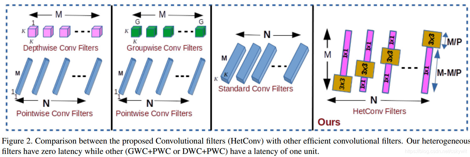
当然CNN训练中的trick不只是这几样，在这里只是简要列出几种成名已久的。最新的CVPR2019中有一篇论文《HetConv: Heterogeneous Kernel-Based Convolutions for Deep CNNs》也很有新意，直接在同一个卷积核内部使用不同的卷积，根据文章所说在准确性不降低的情况下，可以大幅度的减少FLOPS，如图所示，但论文没有提供源码，有时间实现以下发出来。