卷积神经网络
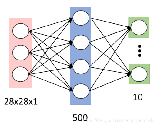
全连接网络的局限性
对于MNIST 手写数字识别,假如第一个隐层的节点数为500,那么一个全连接层的参数个数为:28×28×1×500+500 ≈ 40万。
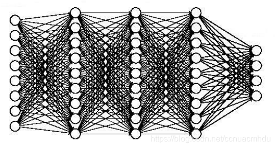
当图片分辨率进一步提高时,当隐层数量增加时,例如:600 x 600 图像,各隐层节点数分别为300,200和100,则参数个数为:600 x 600 x 300 + 300 x 200 + 200 x 100≈ 1.08亿。
参数增多会导致:
计算速度减慢
过拟合
卷积神经网络结构
1962年Hubel和Wiesel通过对猫视觉皮层细胞的研究,提出了感受野的概念。视觉皮层的神经元就是局部接受信息,只受某些特定区域刺激的响应,而不是对全局图像进行感知。
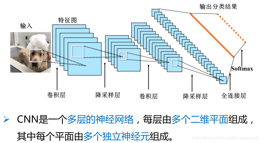
输入层→(卷积层+→池化层?)+→全连接层+
(1)输入层:将每个像素代表一个特征节点输入到网络中。
(2)卷积层:卷积运算的主要目的是使原信号特征增强,并降低噪音。
(3)降采样层:降低网络训练参数及模型的过拟合程度。
(4)全连接层:对生成的特征进行加权。
卷积
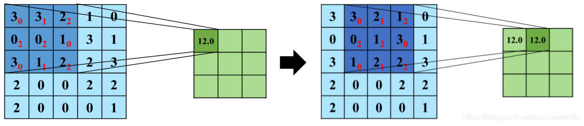
3 x 0 + 3 x 1 + 2 x 2 + 0 x 2 + 0 x 2 + 1 x 0 + 3 x 0 + 1 x 1 + 2 x 2 = 12
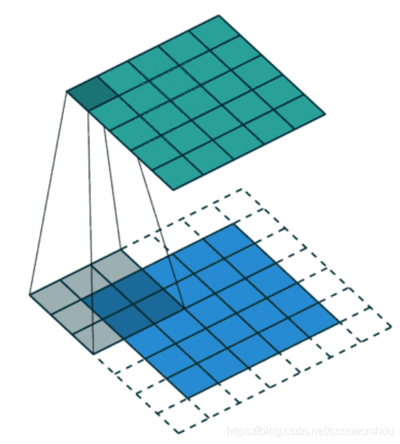
- 卷积核在 2 维输入数据上“滑动”,对当前输入部分的元素进行矩阵乘法,然后将结果汇为单个输出像素值,重复这个过程直到遍历整张图像,这个过程就叫做卷积。
- 这个权值矩阵就是卷积核。
- 卷积操作得到的图像称为特征图(feature map)。
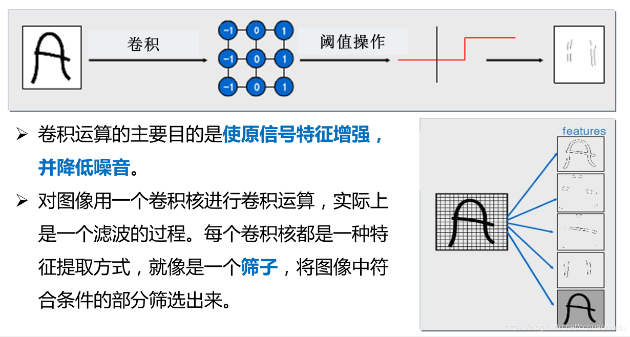
每个卷积核都会将图像生成为另一幅特征映射图,即:一个卷积核提取一种特征。
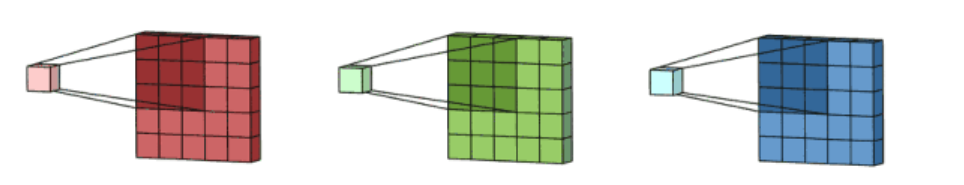
为了使特征提取更充分,可以添加多个卷积核以提取不同的特征,也就是,多通道卷积。
0填充(Padding)
如何使得输出尺寸与输入保持一致呢?扩充边界,边界都填0值像素。
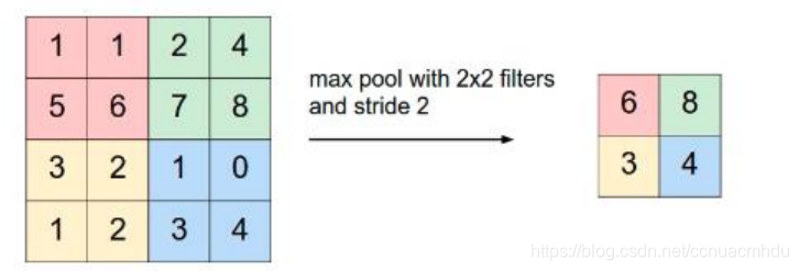
降采样
池化是降采样的一种手段,其实步长大于1的卷积也能达到降采样的效果。
(1) 均值池化:对池化区域内的像素点取均值,这种方法得到的特征数据对背景信息更敏感。
(2) 最大池化:对池化区域内所有像素点取最大值,这种方法得到的特征对纹理特征信息更加敏感。

步长(stride)

tensorflow相关函数
tf.nn.dropout
With probability rate, drops elements of x. Input that are kept are scaled up by 1 / (1 - rate), otherwise outputs 0. The scaling is so that the expected sum is unchanged.(丢掉x中rate比例的元素。没掉丢的输入扩大为1/(1-rate)倍,丢掉的元素值变为0。这个缩放,期望和不变。)
利用MNIST数据集训练卷积神经网络模型
#coding:utf-8
%matplotlib notebook
import tensorflow as tf
from tensorflow.examples.tutorials.mnist import input_data
from time import time
import matplotlib.pyplot as plt
import numpy as np
import os
tf.reset_default_graph()
logDir = "C:\\Users\\20191027\\Documents\\log" # 输出日志,用于TensorBoard可视化
## 1. 准备数据
mnist = input_data.read_data_sets('MNIST_data',one_hot=True)
x = tf.placeholder(tf.float32, [None,784])
y = tf.placeholder(tf.float32,[None,10])
# 转为4D的向量[batch,in_height,in_width,in_channels],batch代表图片数目
x_image = tf.reshape(x, [-1,28,28,1])
## 2. 构建模型
# 初始化权重
def weight_variable(shape):
initial = tf.truncated_normal(shape, stddev=0.1) # 生成一个截断的正态分布
return tf.Variable(initial)
# 初始化偏置
def biases_variable(shape):
initial = tf.constant(0.1, shape=shape)
return tf.Variable(initial)
# 卷基层
def conv2d(x,W):
# x input tensor of shape [batch, in_height, in_width, in_channel]
# W 卷积核 filter / kernel tensor of shape [filter_height, filter_width, in_channels, out_channels]
# strides 步长 strides[0] = strides[3] = 1, strides[1]代表x方向的步长,strides[2]代表y方向的步长
# padding 'SAME' 表示边界填充0像素,保证卷积后的图像大小不变。'VALID' 表示不填充边界。
return tf.nn.conv2d(x,W,strides=[1,1,1,1],padding='SAME')
# 池化层(降采样)
def max_pool_2x2(x):
# ksize [1, x, y, 1] 池化窗口大小
return tf.nn.max_pool(x,ksize=[1,2,2,1],strides=[1,2,2,1],padding='SAME')
# 第一个卷基层
W_conv1 = weight_variable([5,5,1,32]) # 5*5的采样窗口,32个卷积核,抽取32种特征
b_conv1 = biases_variable([32]) # 32个卷积核对应的32个偏置
h_conv1 = tf.nn.relu(conv2d(x_image,W_conv1)+b_conv1) # 卷积操作,并用relu激活
h_pool1 = max_pool_2x2(h_conv1) # 池化操作
# 第二个卷基层
W_conv2 = weight_variable([5,5,32,64]) # 5*5的采样窗口,输入5*5大小的32张图(相当于32通道),输出64种特征图
b_conv2 = biases_variable([64]) # 64个卷积核对应的64个偏置
h_conv2 = tf.nn.relu(conv2d(h_pool1,W_conv2) + b_conv2) # 卷积操作,并用relu激活
h_pool2 = max_pool_2x2(h_conv2) # 池化操作
# 28x28图片第一次卷积后28x28,第一次池化后14x14,
# 第二次卷积后14x14,第二次池化后7x7,
# 上面操作后64张7x7的平面。
# 第一个全连接层
W_fc1 = weight_variable([7*7*64,128]) # 上一层有7*7*64个神经元,全连接层有128个神经元
b_fc1 = biases_variable([128]) # 128个偏执值
h_pool2_flat = tf.reshape(h_pool2,[-1,7*7*64]) # 第二个池化层的输出扁平化为一维
h_fc1 = tf.nn.relu(tf.matmul(h_pool2_flat,W_fc1)+b_fc1) # 求第一个全连接层的输出
# keep_prob用来表示神经元的输出概率
keep_prob = tf.placeholder(tf.float32)
h_fc1_drop = tf.nn.dropout(h_fc1,keep_prob)
# 第二个全连接层
W_fc2 = weight_variable([128,10])
b_fc2 = biases_variable([10])
# 输出
forward = tf.matmul(h_fc1_drop,W_fc2) + b_fc2
prediction = tf.nn.softmax(forward)
# 交叉熵损失函数
cross_entropy = tf.reduce_mean(tf.nn.softmax_cross_entropy_with_logits(labels=y,logits=forward))
## 3. 训练模型
train_epochs = 10
batch_size = 100 # 每个批次的大小
n_batch = mnist.train.num_examples // batch_size # 总批次
learning_rate = 0.001
ckpt_dir = "./ckpt_dir/cnn/" # 保存模型的路径
if not os.path.exists(ckpt_dir):
os.makedirs(ckpt_dir)
# 优化器
optimizer = tf.train.AdamOptimizer(learning_rate).minimize(cross_entropy)
# 准确率
correct_prediction = tf.equal(tf.argmax(prediction,1),tf.argmax(y,1))
accuracy = tf.reduce_mean(tf.cast(correct_prediction,tf.float32))
# 声明完所有变量后,再调用Saver,用于保存模型
saver = tf.train.Saver()
startTime = time()
loss_list = [] # 统计训练每轮的损失
acc_list = [] # 统计训练每轮的准确率
# 训练时间比较久。。。
with tf.Session() as sess:
sess.run(tf.global_variables_initializer())
for epoch in range(train_epochs):
for batch in range(n_batch):
batch_xs,batch_ys = mnist.train.next_batch(batch_size)
sess.run(optimizer,feed_dict={x:batch_xs,y:batch_ys,keep_prob:0.7})
loss, acc = sess.run([cross_entropy, accuracy],
feed_dict={x:mnist.validation.images,
y:mnist.validation.labels,
keep_prob:1.0})
loss_list.append(loss)
acc_list.append(acc)
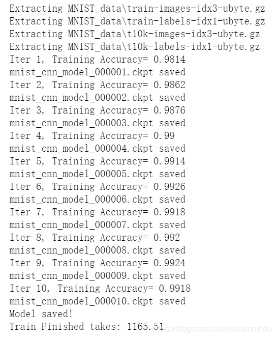
print ("Iter "+ str(epoch+1) + ", Training Accuracy= " + str(acc))
# 保存模型
saver.save(sess, os.path.join(ckpt_dir,'mnist_cnn_model_{:06d}.ckpt'.format(epoch+1)))
print('mnist_cnn_model_{:06d}.ckpt saved'.format(epoch+1))
# 保存最终的模型
saver.save(sess, os.path.join(ckpt_dir, 'mnist_cnn_model.ckpt'))
print("Model saved!")
duration = time() - startTime
print("Train Finished takes:", "{:.2f}".format(duration))
plt.plot(loss_list) # 打印损失随训练轮数的变化曲线
plt.plot(acc_list) # 打印准确率随训练轮数的变化曲线
## 4.预测
acc_test = sess.run(accuracy, feed_dict={x:mnist.test.images,y:mnist.test.labels,keep_prob:1.0})
print("Test Accuarcy:", acc_test)
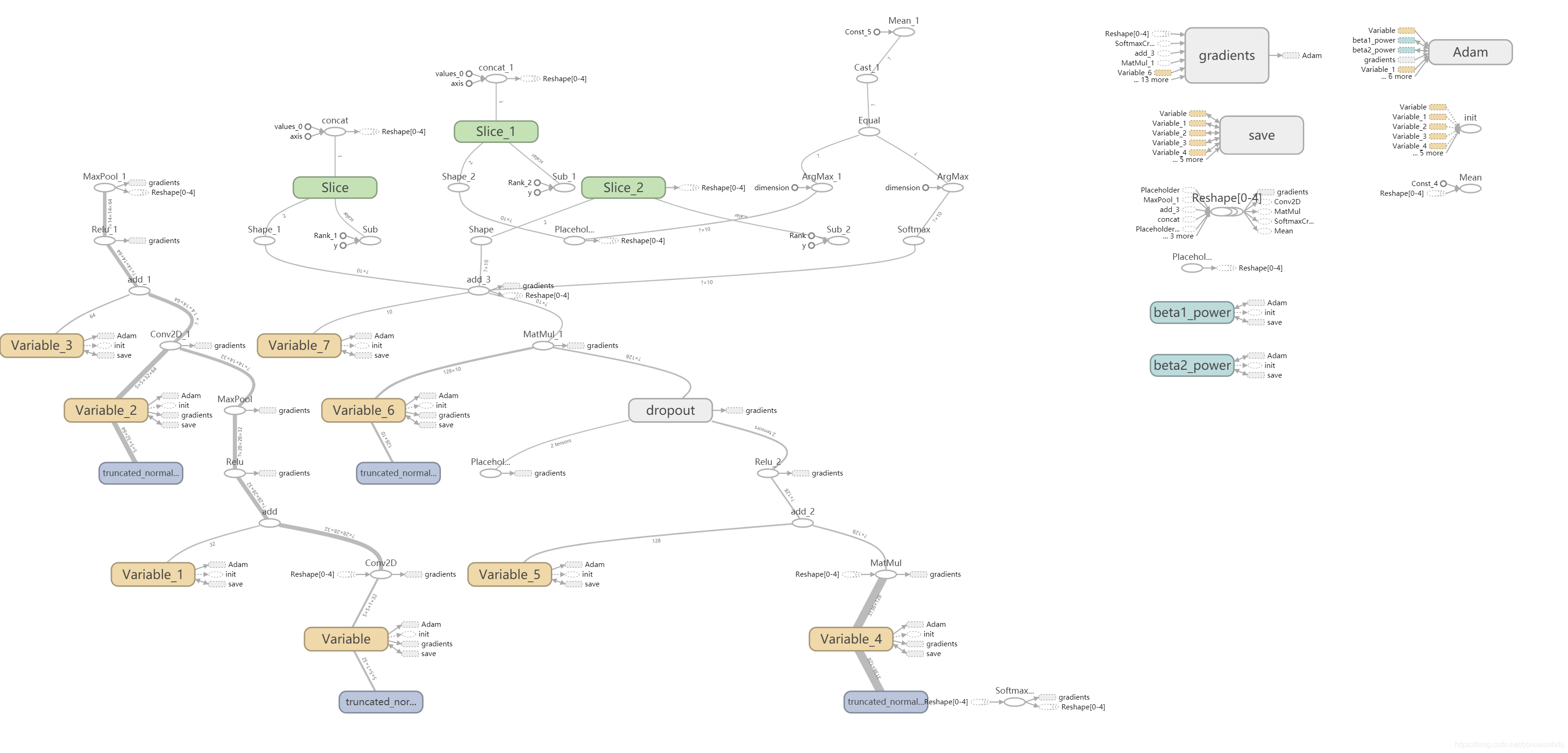
# 输出日志,用于TensorBoard可视化显示
writer = tf.summary.FileWriter(logDir, tf.get_default_graph())
writer.close()

恢复模型
# 恢复CNN模型

import tensorflow as tf
import tensorflow.examples.tutorials.mnist.input_data as input_data

import numpy as np
import matplotlib.pyplot as plt
import cv2

tf.reset_default_graph()

mnist = input_data.read_data_sets('MNIST_data',one_hot=True)

x = tf.placeholder(tf.float32, [None,784])
y = tf.placeholder(tf.float32,[None,10])

# 转为4D的向量[batch,in_height,in_width,in_channels],batch代表图片数目
x_image = tf.reshape(x, [-1,28,28,1])

# 初始化权重
def weight_variable(shape):
    initial = tf.truncated_normal(shape, stddev=0.1)  # 生成一个截断的正态分布
    return tf.Variable(initial)

# 初始化偏置
def biases_variable(shape):
    initial = tf.constant(0.1, shape=shape)
    return tf.Variable(initial)

# 卷基层
def conv2d(x,W):
    # x input tensor of shape [batch, in_height, in_width, in_channel]
    # W 卷积核 filter / kernel tensor of shape [filter_height, filter_width, in_channels, out_channels]
    # strides 步长 strides[0] = strides[3] = 1, strides[1]代表x方向的步长,strides[2]代表y方向的步长
    # padding 'SAME' 表示边界填充0像素,保证卷积后的图像大小不变。'VALID' 表示不填充边界。
    return tf.nn.conv2d(x,W,strides=[1,1,1,1],padding='SAME')

# 池化层(降采样)
def max_pool_2x2(x):
    # ksize [1, x, y, 1] 池化窗口大小
    return tf.nn.max_pool(x,ksize=[1,2,2,1],strides=[1,2,2,1],padding='SAME')


# 第一个卷基层
W_conv1 = weight_variable([5,5,1,32]) # 5*5的采样窗口,32个卷积核,抽取32种特征
b_conv1 = biases_variable([32])  # 32个卷积核对应的32个偏置

h_conv1 = tf.nn.relu(conv2d(x_image,W_conv1)+b_conv1) # 卷积操作,并用relu激活
h_pool1 = max_pool_2x2(h_conv1) # 池化操作

# 第二个卷基层
W_conv2 = weight_variable([5,5,32,64]) # 5*5的采样窗口,输入5*5大小的32张图(相当于32通道),输出64种特征图
b_conv2 = biases_variable([64]) # 64个卷积核对应的64个偏置

h_conv2 = tf.nn.relu(conv2d(h_pool1,W_conv2) + b_conv2) # 卷积操作,并用relu激活
h_pool2 = max_pool_2x2(h_conv2) # 池化操作

# 28x28图片第一次卷积后28x28,第一次池化后14x14,
# 第二次卷积后14x14,第二次池化后7x7,
# 上面操作后64张7x7的平面。

# 第一个全连接层
W_fc1 = weight_variable([7*7*64,128]) # 上一层有7*7*64个神经元,全连接层有128个神经元
b_fc1 = biases_variable([128]) # 128个偏执值

h_pool2_flat = tf.reshape(h_pool2,[-1,7*7*64]) # 第二个池化层的输出扁平化为一维
h_fc1 = tf.nn.relu(tf.matmul(h_pool2_flat,W_fc1)+b_fc1) # 求第一个全连接层的输出

# keep_prob用来表示神经元的输出概率
keep_prob  = tf.placeholder(tf.float32)
h_fc1_drop = tf.nn.dropout(h_fc1,keep_prob)

# 第二个全连接层
W_fc2 = weight_variable([128,10])
b_fc2 = biases_variable([10])

# 输出
forward = tf.matmul(h_fc1_drop,W_fc2) + b_fc2
prediction = tf.nn.softmax(forward)

# 准确率
correct_prediction = tf.equal(tf.argmax(prediction,1),tf.argmax(y,1))
accuracy = tf.reduce_mean(tf.cast(correct_prediction,tf.float32))

ckpt_dir = "./ckpt_dir/cnn/" # 保存模型的路径

saver = tf.train.Saver()

sess = tf.Session()
sess.run(tf.global_variables_initializer())

ckpt = tf.train.get_checkpoint_state(ckpt_dir)

if ckpt and ckpt.model_checkpoint_path:
    saver.restore(sess, ckpt.model_checkpoint_path)
    print("Restore model from "+ckpt.model_checkpoint_path)

# 预测
print("Test Accuracy:", accuracy.eval(session=sess,
                                      feed_dict={x:mnist.test.images, y:mnist.test.labels, keep_prob:1.0}))
