一、Dijkstra算法
Dijkstra算法从物体所在的初始点开始,访问图中的结点。它迭代检查待检查结点集中的结点,并把和该结点最靠近的尚未检查的结点加入待检查结点集。该结点集从初始结点向外扩展,直到到达目标结点。Dijkstra算法保证能找到一条从初始点到目标点的最短路径,只要所有的边都有一个非负的代价值。
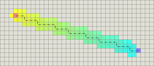
1.1 算法原理与效果图
Dijkstra算法采用贪心算法的思想,解决的问题可以描述为:在无向图 G=(V,E) 中,假设每条边 E[i] 的长度为 w[i],找到由顶点vs到其余各点的最短路径。
通过Dijkstra计算图G中的最短路径时,需要指定起点vs(即从顶点vs开始计算)。此外,引进两个集合S和U。S的作用是记录已求出最短路径的顶点(以及相应的最短路径长度),而U则是记录还未求出最短路径的顶点(以及该顶点到起点vs的距离)。初始时,S中只有起点vs;U中是除vs之外的顶点,并且U中顶点的路径是"起点vs到该顶点的路径"。然后,从U中找出路径最短的顶点,并将其加入到S中;接着,更新U中的顶点和顶点对应的路径。 然后,再从U中找出路径最短的顶点,并将其加入到S中;接着,更新U中的顶点和顶点对应的路径。重复该操作,直到遍历完所有顶点。

1.2 源码分析
源码来自:https://github.com/AtsushiSakai/PythonRobotics/blob/master/PathPlanning/Dijkstra/dijkstra.py
算法实现的主代码分析:
def dijkstra_planning(sx, sy, gx, gy, ox, oy, reso, rr):
    """
    sx: start x position [m]
    sy: start y position [m]          #起始点坐标
    gx: goal x position [m]
    gy: goal y position [m]           #目标点坐标
    ox: x position list of Obstacles [m]
    oy: y position list of Obstacles [m]   #障碍点坐标
    reso: grid resolution [m]          #栅格地图分辨率
    rr: robot radius[m]                      #机器人的半径
    """

    nstart = Node(round(sx / reso), round(sy / reso), 0.0, -1)  # 同除地图分辨率,坐标四舍五入后归一化
    ngoal = Node(round(gx / reso), round(gy / reso), 0.0, -1)
    ox = [iox / reso for iox in ox]
    oy = [ioy / reso for ioy in oy]

    obmap, minx, miny, maxx, maxy, xw, yw = calc_obstacle_map(ox, oy, reso, rr)  # 障碍物地图范围计算、保存

    motion = get_motion_model()  # 节点移动向量共8组对应8个移动方向(x,y,cost)

    openset, closedset = dict(), dict()  # 创建openset和closedset,分别存放未找到和已找到的路径点
    openset[calc_index(nstart, xw, minx, miny)] = nstart

    while 1:
        c_id = min(openset, key=lambda o: openset[o].cost)  # 找到openlist中离出发点最近的点
        current = openset[c_id]


        # 画图,画出当前路径点
        if show_animation:
            plt.plot(current.x * reso, current.y * reso, "xc")
            if len(closedset.keys()) % 10 == 0:
                plt.pause(0.001)


     # 如果到达目标点,结束循环
        if current.x == ngoal.x and current.y == ngoal.y:
            print("Find goal")
            ngoal.pind = current.pind
            ngoal.cost = current.cost
            break

        # 将符合要求的路径点移出openlist
        del openset[c_id]
        # 将符合要求的路径点添加进closedlist
        closedset[c_id] = current

        # 基于移动向量,扩大搜索范围
        for i, _ in enumerate(motion):
            node = Node(current.x + motion[i][0], current.y + motion[i][1],
                        current.cost + motion[i][2], c_id)
            n_id = calc_index(node, xw, minx, miny)


       # 如果新的路径点不符合要求,结束本次循环
            if not verify_node(node, obmap, minx, miny, maxx, maxy):
                continue

       # 如果新的路径点已经在closedlist中,结束本次循环
            if n_id in closedset:
                continue
            # 如果新的路径点在openlist中,
            if n_id in openset:
                if openset[n_id].cost > node.cost:
                    openset[n_id].cost = node.cost
                    openset[n_id].pind = c_id  #pind类似于指针的作用,指向当前节点的上一节点,方便最后进行路径回溯
            else:
                openset[n_id] = node  #向openlist中添加新的路径点

    rx, ry = calc_final_path(ngoal, closedset, reso)  #rx,ry为数组,存放着满足条件的路径节点

    return rx, ry
二、A*算法
BFS算法按照与Dijkstra算法类似的流程运行,不同的是它能够评估任意节点到达目标点的代价。与Dijkstra算法选择离初始节点最近的节点不同,它选择离目标最近的节点。BFS算法不能保证找到一条最短路径,但速度比Dijkstra速度快很.A*算法就是结合了BFS算法和Dijkstra算法,具有了启发式方法的特性,且能保证找到一条最短路径。
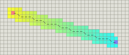
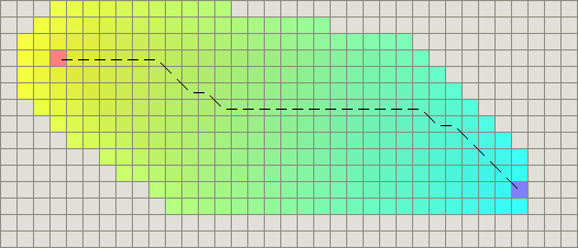
2.1 算法原理与效果图
-
启发式搜素:启发式搜索就是在状态空间中的搜索对每一个搜索的位置进行评估,得到最好的位置,再从这个位置进行搜索直到目标。这样可以省略大量无畏的搜索路径,提到了效率。在启发式搜索中,对位置的估价是十分重要的。采用了不同的估价可以有不同的效果
- 估值函数(cost):从当前节点移动到目标节点的预估费用;这个估计就是启发式的。在寻路问题和迷宫问题中,通常用曼哈顿(manhattan)估价函数预估费用
- start:路径规划的起始点
- goal:路径规划的终点
- g_score:从当前点(current_node)到出发点(start)的移动代价
- h_score:不考虑障碍物,从当前点(current_node)到目标点的估计移动代价
- f_score:f_score=g_score+h_score
- openlist:寻路过程中的待检索节点列表
- closelist:不需要再次检索的节点列表
- comaFrom:存储父子节点关系的列表,用于回溯最优路径,非必须,也可以通过节点指针实现
2.2 源码分析
源码来自:https://github.com/AtsushiSakai/PythonRobotics/blob/master/PathPlanning/AStar/a_star.py
主要代码内容与Dijkstra相似,增加了基于欧几里得距离的calc_heuristic()函数:
def a_star_planning(sx, sy, gx, gy, ox, oy, reso, rr):
    """
    gx: goal x position [m]
    gy: goal y position [m]
    ox: x position list of Obstacles [m]
    oy: y position list of Obstacles [m]
    reso: grid resolution [m]
    rr: robot radius[m]
    """

    nstart = Node(round(sx / reso), round(sy / reso), 0.0, -1)
    ngoal = Node(round(gx / reso), round(gy / reso), 0.0, -1)
    ox = [iox / reso for iox in ox]
    oy = [ioy / reso for ioy in oy]

    obmap, minx, miny, maxx, maxy, xw, yw = calc_obstacle_map(ox, oy, reso, rr)

    motion = get_motion_model()

    openset, closedset = dict(), dict()
    openset[calc_index(nstart, xw, minx, miny)] = nstart

    while 1:
        c_id = min(openset, key=lambda o: openset[o].cost + calc_heuristic(ngoal, openset[o])) #对应于F=G+H
        current = openset[c_id]

        # show graph
        if show_animation:  # pragma: no cover
            plt.plot(current.x * reso, current.y * reso, "xc")
            if len(closedset.keys()) % 10 == 0:
                plt.pause(0.001)

        if current.x == ngoal.x and current.y == ngoal.y:
            print("Find goal")
            ngoal.pind = current.pind
            ngoal.cost = current.cost
            break

        # Remove the item from the open set
        del openset[c_id]
        # Add it to the closed set
        closedset[c_id] = current

        # expand search grid based on motion model
        for i, _ in enumerate(motion):
            node = Node(current.x + motion[i][0],
                        current.y + motion[i][1],
                        current.cost + motion[i][2], c_id)
            n_id = calc_index(node, xw, minx, miny)

            if n_id in closedset:
                continue

            if not verify_node(node, obmap, minx, miny, maxx, maxy):
                continue

            if n_id not in openset:
                openset[n_id] = node  # Discover a new node
            else:
                if openset[n_id].cost >= node.cost:
                    # This path is the best until now. record it!
                    openset[n_id] = node

    rx, ry = calc_final_path(ngoal, closedset, reso)

    return rx, ry
增加的calc_heuristic()函数:
def calc_heuristic(n1, n2):
    w = 1.0  # weight of heuristic(H函数的权重)
    d = w * math.sqrt((n1.x - n2.x)**2 + (n1.y - n2.y)**2)  #欧几里得距离计算
    return d
2.3 网格地图中的启发式算法
- 曼哈顿距离:
标准的启发式函数是曼哈顿距离(Manhattan distance)。考虑你的代价函数并找到从一个位置移动到邻近位置的最小代价D。因此,地图中的启发式函数应该是曼哈顿距离的D倍,常用于在地图上只能前后左右移动的情况:
H(n) = D * (abs ( n.x – goal.x ) + abs ( n.y – goal.y ) )
- 对角线距离:
如果在你的地图中你允许对角运动那么你需要一个不同的启发函数。(4 east, 4 north)的曼哈顿距离将变成8*D。然而,你可以简单地移动(4 northeast)代替,所以启发函数应该是4*D。这个函数使用对角线,假设直线和对角线的代价都是D:
h(n) = D * max(abs(n.x - goal.x), abs(n.y - goal.y))
- 欧几里得距离:
如果你的单位可以沿着任意角度移动(而不是网格方向),那么你也许应该使用直线距离:
h(n) = D * sqrt((n.x-goal.x)^2 + (n.y-goal.y)^2)
然而,如果是这样的话,直接使用A*时将会遇到麻烦,因为代价函数g不会match启发函数h。因为欧几里得距离比曼哈顿距离和对角线距离都短,你仍可以得到最短路径,不过A*将运行得更久一些:
- 平方后的欧几里得距离:
我曾经看到一些A*的网页,其中提到让你通过使用距离的平方而避免欧几里得距离中昂贵的平方根运算:
h(n) = D * ((n.x-goal.x)^2 + (n.y-goal.y)^2)
不要这样做!这明显地导致衡量单位的问题。当A*计算f(n) = g(n) + h(n),距离的平方将比g的代价大很多,并且你会因为启发式函数评估值过高而停止。对于更长的距离,这样做会靠近g(n)的极端情况而不再计算任何东西,A*退化成BFS:
