文章目录
0、背景
本来这一节其实可以放在《matlab文档查阅使用训练(手把手教你阅读matlab文档)全网首发原创》,但是由于这两个函数非常重要,所以想单独拿出来记录,以便后续使用。
1、chrip信号
A chirp is a signal in which the frequency increases (up-chirp) or decreases (down-chirp) with time. In some sources, the term chirp is used interchangeably with sweep signal. It is commonly used in sonar and radar, but has other applications, such as in spread-spectrum communications.
chirp是频率随时间增加或减小的一种信号。在某些领域中,chirp这个词可以与扫频信号的名词互换使用。通常用于雷达,声呐中,但是也有别的用途,例如扩频通信。

1、matlab帮助文档对chirp的解释

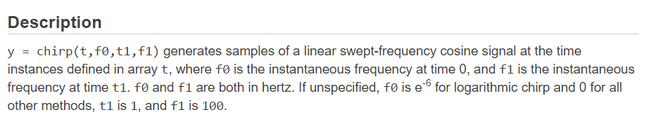
从上面描述可以知道,一般来说我们常用的syntax的第一种形式,其中t是变量,包含了我们的时间点数(采样率),而f0和t1以及f1都是固定的,f0代表了在时间0的瞬时频率,f1代表了在时间t1时刻的瞬时频率。
下面是句法2的用法,method可以指定扫频的选项,也就是说,我们也可以非线性扫频。

第二种扫频模式是quadratic,也就是说要求t,是需要开平方根的。

第三种是对数形式,也就是说要求时间,是需要求对数的。

指定凹凸可以使扫频上凸或者凹的频率上升和下降

2、非线性调频
1、高斯包络的调频信号


w = gausswin(N,Alpha)返回一个N点高斯窗口,Alpha与标准差的倒数成正比。窗口的宽度是α的值成反比。更大的α值产生一个窄窗口。α的值默认为2.5。

% Generate a chirp with linear instantaneous frequency deviation.
% The chirp is sampled at 1 kHz for 2 seconds.
% The instantaneous frequency is 0 at t = 0 and crosses 250 Hz at t = 1 second.

clc
clear
close all


t = 0:1/1e3:1;      %以1KHZ的频率采样2秒钟
y = chirp(t,0,1,250);
y1=gausswin(length(y),2.5);%默认标准的高斯包络是2.5
y1=y1.';
H=y.*y1;
subplot(3,1,1)
plot(t,y)
subplot(3,1,2)
spectrogram(y,256,250,256,1e3,'yaxis')
subplot(3,1,3)
plot(t,H);
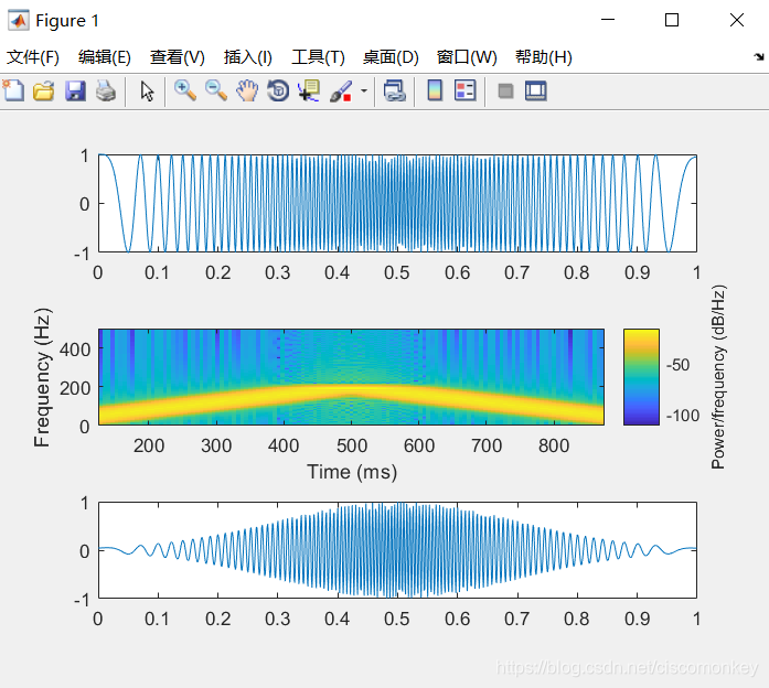
现在,我要产生一个高斯包络的线性调频信号,但是频率逐渐增高,到了中间点,频率达到最高,然后频率在逐渐减小,以中间为对称。
clc
clear
close all


t1 = 0:1/1e3:(1-1/1e3)/2;      %以1KHZ的频率采样0.5秒钟
y1 = chirp(t1,0,(1-1/1e3)/2,200);
y2 = chirp(t1,200,(1-1/1e3)/2,0);
y=[y1,y2];
t=[t1,t1+0.499000000000000+1/1e3];
g=gausswin(length(y),2.5);%默认标准的高斯包络是2.5
g=g.';
H=y.*g;
subplot(3,1,1)
plot(t,y)
subplot(3,1,2)
spectrogram(y,256,250,256,1e3,'yaxis')
subplot(3,1,3)
plot(t,H);
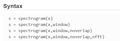
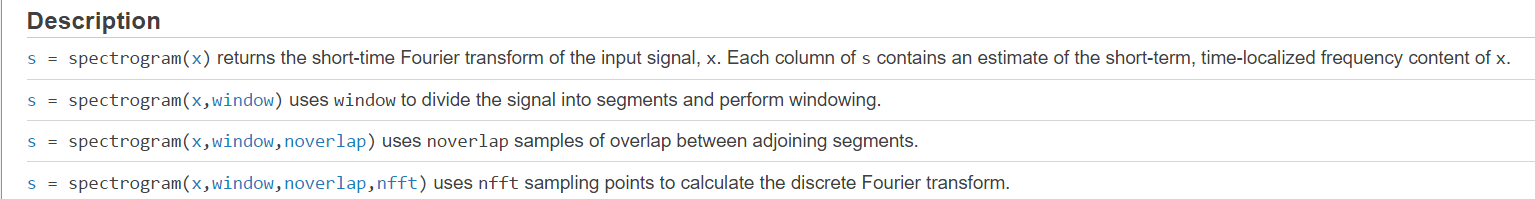
2、spectrogram

- s=spectrogram(x)
表示将x进行默认的短时傅里叶变换,默认窗口使用海明窗,将x分成8段。
如果x不能被平分成8段,则会做截断处理。默认情况下,其他参数的默认值为
window—窗函数,默认为nfft长度的海明窗Hamming
noverlap—每一段的重叠样本数,默认值是在各段之间产生50%的重叠
nfft—做FFT变换的长度,默认为256和大于每段长度的最小2次幂之间的最大值。
另外,此参数除了使用一个常量外,还可以指定一个频率向量F
fs—采样频率,默认值归一化频率
案例:
Generate samples of a signal that consists of a sum of sinusoids. The normalized frequencies of the sinusoids are rad/sample and rad/sample. The higher frequency sinusoid has 10 times the amplitude of the other sinusoid.
产生一个正弦曲线,归一化频率都是rad/sample,更高的频率的正弦信号是低正弦信号幅度的10倍。
正弦信号1:2π/5;
正弦信号2: 4π/5;
 N = 1024;
n = 0:N-1;

w0 = 2*pi/5;
x = sin(w0*n)+10*sin(2*w0*n);
%Compute the short-time Fourier transform using the function defaults. Plot the spectrogram.

s = spectrogram(x);

spectrogram(x,'yaxis')

- Power Spectral Densities of Chirps
Compute and display the PSD of each segment of a quadratic chirp that starts at 100 Hz and crosses 200 Hz at t = 1 s. Specify a sample rate of 1 kHz, a segment length of 128 samples, and an overlap of 120 samples. Use 128 DFT points and the default Hamming window.
计算chirp信号的功率谱,chirp信号以频率100HZ到200HZ,指定采样率是1KHZ,一段的采样长度是128个点,overlap是120个点,使用128点的DFT,采用默认的汉明窗。
clc;
clear;
t = 0:0.001:2;
x = chirp(t,100,1,200,'quadratic');

spectrogram(x,128,120,128,1e3,'yaxis')
title('Quadratic Chirp')

也就是说,在时间域上,分为了t/8, 这么多个时间段,因为非覆盖部分是128-120。时间片段分的越细,频率随着时间的变化也就越精确。
下面我们来看看,overlap不重叠。下面就是将时间分为了15段。精度是比较差的。

下面再看一个实例
Compute and display the PSD of each segment of a linear chirp that starts at DC and crosses 150 Hz at t = 1 s. Specify a sample rate of 1 kHz, a segment length of 256 samples, and an overlap of 250 samples. Use the default Hamming window and 256 DFT points.
计算并且展示每一段线性chirp信号的PSD,这个信号从直流到在时间1s的时候150HZ,指定采样率是1KHZ,每一段的长度是256个采样点,overlap为250个,使用默认的汉明窗口,做256个点的DFT。

上面我们就已经把基本的用法都讲解完毕了
下面,我们来看返回参数的spectrogram

其实,我们只要会这句有参数返回值的语法就好:
[S,F,T,P]=spectrogram(x,window,noverlap,nfft,fs)
参考:
https://blog.csdn.net/zhuguorong11/article/details/77801977
clc;
clear;
N = 1024;
n = 0:N-1;


t = 0:0.001:2-0.001;
x = chirp(t,0,1,150,'li');
[s,f,T,p]=spectrogram(x,128,120,128,1e3,'yaxis');
figure;
plot(x);
figure;
spectrogram(x,128,120,128,1e3,'yaxis');
title('linear Chirp')

k = fix((length(x)-120)/(128-120))
k =235
搞懂参数返回值的意义后,我们再来看如何利用参数返回值进行画图
clc;
clear;
t = 0:0.001:2-0.001;
x = chirp(t,0,1,150,'li');
[s,f,T,p]=spectrogram(x,128,120,128,1e3,'yaxis');
figure;
plot(x);
figure;
surf(T,f,10*log10(p),'edgecolor','none'); axis tight;
title('linear Chirp');
xlabel('Time (Seconds)'); ylabel('Hz');
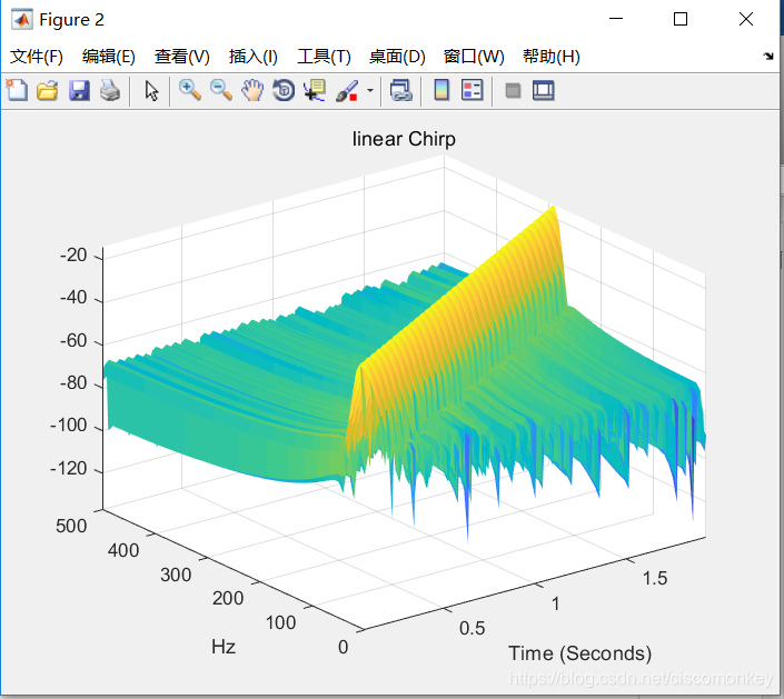
这里我们要讲解一下,这里我们已经得到了返回参数值S F T P 。这四个参数的含义,就不必多说了,具体参考发的链接。
下面看一下surf这个函数。
利用surf根据spectrogram的返回参数值绘制三维

surf(X,Y,Z) creates a three-dimensional surface plot. The function plots the values in matrix Z as heights above a grid in the x-y plane defined by X and Y. The function also uses Z for the color data, so color is proportional to height.
这个函数用于绘制三维图,这个函数绘制以Z为高度,以X-Y为平面,这个函数使用Z为颜色数据。
surf(___,Name,Value) specifies surface properties using one or more name-value pair arguments. For example, ‘FaceAlpha’,0.5 creates a semitransparent surface. Specify name-value pairs after all other input arguments.
surf(,Name,Value)使用一个或多个名称-值对参数指定表面属性。例如,‘FaceAlpha’,0.5创建一个半透明的表面。在所有其他输入参数之后指定名称-值对。
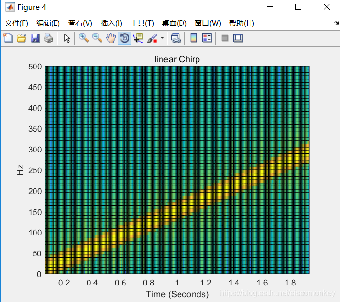
下图是仅仅使用
surf(T,f,10*log10§);
也就是说以时间轴T为X轴,f为频率轴,功率谱是10log10§.
Use s to access and modify properties of the surface object after it is created. For example, turn off the display of the edges by setting the EdgeColor property.
s.EdgeColor = ‘none’;
使用上述edgecolor可以关闭边缘线。
clc;
clear;
t = 0:0.001:2-0.001;
x = chirp(t,0,1,150,'li');
[s,f,T,p]=spectrogram(x,128,120,128,1e3,'yaxis');
figure;
plot(x);
figure;
Q=surf(T,f,10*log10(p)); axis tight;
Q.EdgeColor='none';
title('linear Chirp');
xlabel('Time (Seconds)'); ylabel('Hz');
