决策树-基于opencv和python的学习笔记（十七）

版权声明：本文为博主原创文章，未经博主允许不得转载。https://blog.csdn.net/weixin_44474718/article/details/86830184

决策树是一个简单但有效的监督学习算法。

一、构建第一个决策树

import matplotlib.pyplot as plt
plt.style.use('ggplot')
from sklearn.feature_extraction import DictVectorizer
import numpy as np
import sklearn.model_selection as ms
import cv2
from sklearn import metrics
from sklearn import tree
import pydotplus

# 20个不同病人的数据
data = [
    {'age': 33, 'sex': 'F', 'BP': 'high', 'cholesterol': 'high', 'Na': 0.66, 'K': 0.06, 'drug': 'A'},
    {'age': 77, 'sex': 'F', 'BP': 'high', 'cholesterol': 'normal', 'Na': 0.19, 'K': 0.03, 'drug': 'D'},
    {'age': 88, 'sex': 'M', 'BP': 'normal', 'cholesterol': 'normal', 'Na': 0.80, 'K': 0.05, 'drug': 'B'},
    {'age': 39, 'sex': 'F', 'BP': 'low', 'cholesterol': 'normal', 'Na': 0.19, 'K': 0.02, 'drug': 'C'},
    {'age': 43, 'sex': 'M', 'BP': 'normal', 'cholesterol': 'high', 'Na': 0.36, 'K': 0.03, 'drug': 'D'},
    {'age': 82, 'sex': 'F', 'BP': 'normal', 'cholesterol': 'normal', 'Na': 0.09, 'K': 0.09, 'drug': 'C'},
    {'age': 40, 'sex': 'M', 'BP': 'high', 'cholesterol': 'normal', 'Na': 0.89, 'K': 0.02, 'drug': 'A'},
    {'age': 88, 'sex': 'M', 'BP': 'normal', 'cholesterol': 'normal', 'Na': 0.80, 'K': 0.05, 'drug': 'B'},
    {'age': 29, 'sex': 'F', 'BP': 'high', 'cholesterol': 'normal', 'Na': 0.35, 'K': 0.04, 'drug': 'D'},
    {'age': 53, 'sex': 'F', 'BP': 'normal', 'cholesterol': 'normal', 'Na': 0.54, 'K': 0.06, 'drug': 'C'},
    {'age': 36, 'sex': 'F', 'BP': 'high', 'cholesterol': 'high', 'Na': 0.53, 'K': 0.05, 'drug': 'A'},
    {'age': 63, 'sex': 'M', 'BP': 'low', 'cholesterol': 'high', 'Na': 0.86, 'K': 0.09, 'drug': 'B'},
    {'age': 60, 'sex': 'M', 'BP': 'low', 'cholesterol': 'normal', 'Na': 0.66, 'K': 0.04, 'drug': 'C'},
    {'age': 55, 'sex': 'M', 'BP': 'high', 'cholesterol': 'high', 'Na': 0.82, 'K': 0.04, 'drug': 'B'},
    {'age': 35, 'sex': 'F', 'BP': 'normal', 'cholesterol': 'high', 'Na': 0.27, 'K': 0.03, 'drug': 'D'},
    {'age': 23, 'sex': 'F', 'BP': 'high', 'cholesterol': 'high', 'Na': 0.55, 'K': 0.08, 'drug': 'A'},
    {'age': 49, 'sex': 'F', 'BP': 'low', 'cholesterol': 'normal', 'Na': 0.27, 'K': 0.05, 'drug': 'C'},
    {'age': 27, 'sex': 'M', 'BP': 'normal', 'cholesterol': 'normal', 'Na': 0.77, 'K': 0.02, 'drug': 'B'},
    {'age': 51, 'sex': 'F', 'BP': 'low', 'cholesterol': 'high', 'Na': 0.20, 'K': 0.02, 'drug': 'D'},
    {'age': 38, 'sex': 'M', 'BP': 'high', 'cholesterol': 'normal', 'Na': 0.78, 'K': 0.05, 'drug': 'A'}
]
target = [d['drug'] for d in data]               # 将标签保存到target
[d.pop('drug') for d in data]                    #　将data中的标签列去掉
age = [d['age'] for d in data]                   # 提取data中的age
sodium = [d['Na'] for d in data]
potassium = [d['K'] for d in data]
plt.scatter(sodium,potassium)
plt.xlabel('sodium')
plt.ylabel('potassium')
#lt.show()

# 分别根据标签c=target匹配不同的颜色
target = [ord(d) - 65 for d in target]                # 将目标标签中的ABCD转换为数值
plt.subplot(221)
plt.scatter([d['Na'] for d in data], [d['K'] for d in data],c=target, s=100)
plt.xlabel('sodium (Na)')
plt.ylabel('potassium (K)')
plt.subplot(222)
plt.scatter([d['age'] for d in data], [d['K'] for d in data],c=target, s=100)
plt.xlabel('age')
plt.ylabel('potassium (K)')
plt.subplot(223)
plt.scatter([d['age'] for d in data], [d['Na'] for d in data],c=target, s=100)
plt.xlabel('age')
plt.ylabel('sodium (Na)')
#plt.show()

#　数据预处理　　将所有的特征转换为数值特征

vec = DictVectorizer(sparse=False)
data_pre = vec.fit_transform(data)
# print (vec.get_feature_names())        #　得到特征名字
# print (data_pre[0])                    #  特征值
data_pre = np.array(data_pre, dtype = np.float32)        # 保证数据兼容 opencv
target = np.array(target, dtype=np.float32)
x_train , x_test, y_train, y_test = ms.train_test_split(data_pre, target, test_size=5, random_state=42)
"""
# 构建决策树
dtree = cv2.ml.DTrees_create()          # 创建空的决策树   采用opencv方法
dtree.train(x_train, cv2.ml.ROW_SAMPLE, y_train)       # 在训练数据集上训练决策树
y_pred = dtree.predict(x_test)                         # 预测新数据的标签
print (metrics.accuracy_score(y_train, dtree.predict(x_train)))  # 评判决策树性能
print (metrics.accuracy_score(y_test, dtree.predict(x_test)))    #
"""
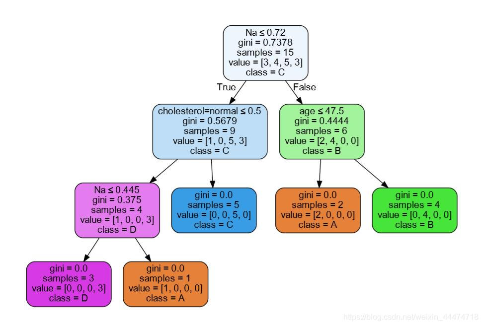
# 可视化训练得到的决策树
dtc = tree.DecisionTreeClassifier()          # 创建空的决策树  采用sklearn方法
dtc.fit(x_train, y_train)                    # 在训练数据集上训练决策树
print (dtc.score(x_train, y_train))
print (dtc.score(x_test , y_test) )

# 保存模型    画图，保存到pdf文件    设置图像参数
with open("tree.pdf", 'w') as doc_data: dot_data = tree.export_graphviz(dtc, out_file=None,
                         feature_names=vec.get_feature_names(),
                         class_names=['A', 'B', 'C', 'D'],
                         filled=True, rounded=True,
                         special_characters=True)
graph = pydotplus.graph_from_dot_data(dot_data)
# 保存图像到pdf文件
graph.write_pdf("tree.pdf")
print (dtc.feature_importances_)           # 特征重要性评分
plt.figure(figsize=(12, 6))                # 画出柱状图
plt.barh(range(10), dtc.feature_importances_, align='center', tick_label=vec.get_feature_names())
plt.show()
dtce = tree.DecisionTreeClassifier(criterion='entropy')     #　指定分割标准

可视化决策树：

Understanding decision rules

Two of the most commonly used criteria for making decisions are the following:

• criterion='gini': The Gini impurity is a measure of misclassification, with the aim of minimizing the probability of misclassification.

• criterion='entropy': In information theory, entropy is a measure of the amount of uncertainty associated with a signal or distribution.

Controlling the complexity of decision trees

There are two common ways to avoid overfitting:

• pre-pruning: This is the process of stopping the creation of the tree early.
• post-pruning (or just pruning): This is the process of first building the tree but then removing or collapsing nodes that contain
  only little information.

There are a number of ways to pre-prune a tree, all of which can be achieved by passing optional arguments to the DecisionTreeClassifier constructor:

• limiting the maximum depth of the tree via the max_depth parameter
• limiting the maximum number of leaf nodes via max_leaf_nodes
• requiring a minimum number of points in a node to keep splitting it
  via min_samples_split

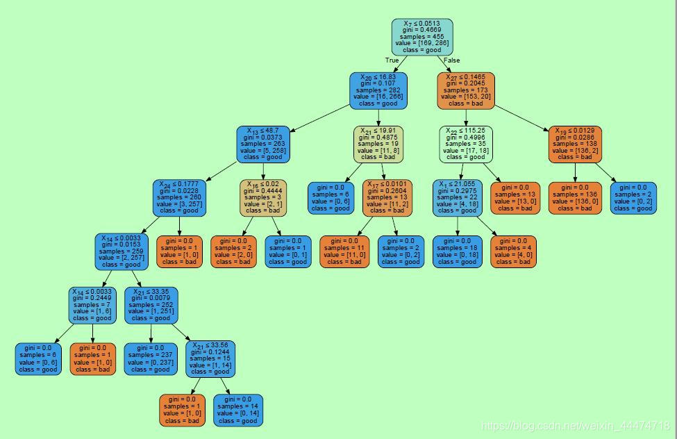
二、使用决策树进行乳腺癌的诊断

二分类问题

In order to make the take feasible, the researchers performed feature extraction on the images, like we did in Chapter 4, Representing Data and Engineering Features. They went through a total of 569 images, and extracted 30 different features that describe the characteristics of the cell nuclei present in the images, including:

• cell nucleus texture (represented by the standard deviation of the
  gray-scale values)

• cell nucleus size (calculated as the mean of distances from center to
  points on the perimeter)

• tissue smoothness (local variation in radius lengths)

• tissue compactness

from sklearn import datasets
import sklearn.model_selection as ms
from sklearn import tree
import pydotplus
import numpy as np
import matplotlib.pyplot as plt
import matplotlib as mpl

data = datasets.load_breast_cancer()     # 载入数据集
"""
print(data.data.shape)
print(data.feature_names)
print(data.target_names)
"""
x_train, x_test, y_train, y_test = ms.train_test_split(data.data, data.target, test_size=0.2, random_state=42)
dtc = tree.DecisionTreeClassifier()     # 创建决策树
dtc.fit(x_train, y_train)               # 训练决策树
print (dtc.score(x_train, y_train))
print (dtc.score(x_test, y_test))
# 保存模型    画图，保存到pdf文件    设置图像参数
with open("tree.pdf", 'w') as doc_data: dot_data = tree.export_graphviz(dtc, out_file=None,
                         class_names=['bad', 'good'],
                         filled=True, rounded=True,
                         special_characters=True)
graph = pydotplus.graph_from_dot_data(dot_data)
graph.write_pdf("tree.pdf")              # 保存图像到pdf文件

# 构建不同的决策树
max_depths = np.array([1,2,3,5,7,9,11])      # 设置不同的决策树深度
train_score=[]
test_score=[]
for d in max_depths:
    dtc= tree.DecisionTreeClassifier(max_depth=d)
    dtc.fit(x_train, y_train)
    train_score.append(dtc.score(x_train , y_train))
    test_score.append(dtc.score(x_test ,y_test))
plt.style.use('ggplot')
plt.figure(figsize=(6,10))
plt.subplot(121)
plt.plot(max_depths,train_score,'o-',linewidth=3, label='train')
plt.plot(max_depths,test_score,'s-',linewidth=3, label='test')
plt.xlabel('max_depths')
plt.ylabel('score')
plt.legend()

train_score2=[]
test_score2=[]
min_samples = np.array([2,4,8,16,32])        # 设置不同的决策树叶节点最小数目
for s in min_samples:
    dtc = tree.DecisionTreeClassifier(min_samples_leaf=s)
    dtc.fit(x_train,y_train)
    train_score2.append(dtc.score(x_train,y_train))
    test_score2.append(dtc.score(x_test,y_test))

plt.subplot(122)
plt.plot(min_samples,train_score2,'o-',linewidth=3, label='train')
plt.plot(min_samples,test_score2,'s-',linewidth=3, label='test')
plt.xlabel('max_depths')
plt.ylabel('score')
plt.legend()
plt.show()

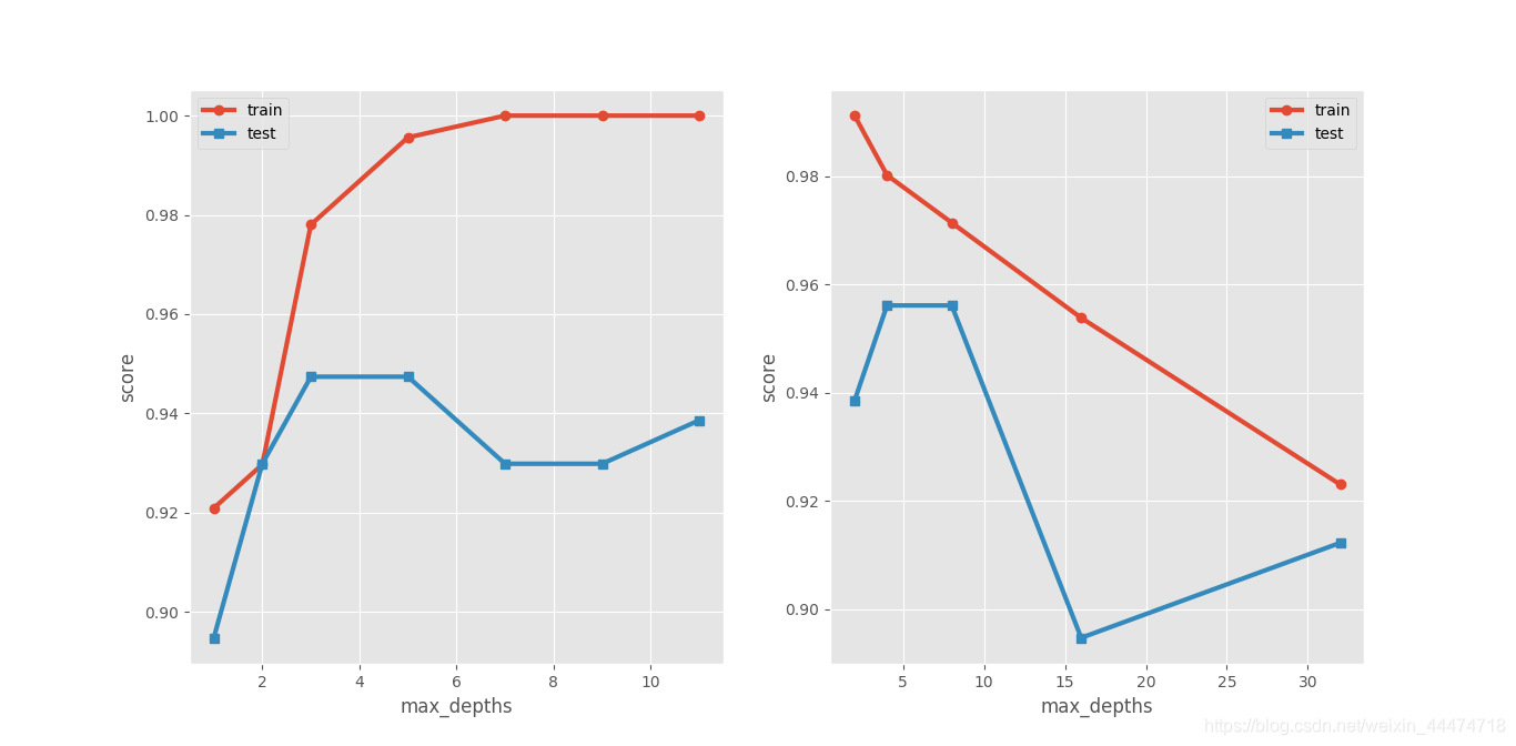
可以通过调参改变决策树的性能。一般在调参过程中，**在训练数据集上的得分有一个单调的关系，要么稳固上升，要么下降。**在测试集上的得分，常常会出现一个上升期，一个局部最大值，之后在测试数据集上的得分将再次开始降低。

一般情况下，预剪枝可以预防过拟合。

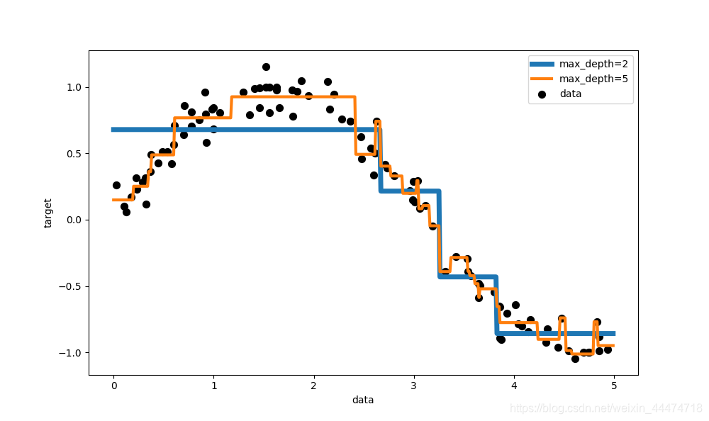
三、使用决策树进行回归

分割标准gini和entropy无法应用到回归中。而是应用 mse（均方误差） 和mae （平均绝对值差）替代。

例1:

a=[0,1,2,3,4,5,6,7]

print(a[1:3:1])输出是[1, 2]，意思是从下标1开始以步长为1到下标3结束

print(a[1:4:2])输出是[1, 3]，意思是从下标1开始以步长为2到下标4结束

例2：

inputs[：，：：2，，：]

意思是：
第一维度，从开始以步长为1到结束

第二维度，从开始以步长为2到结束输出

第三维度，从开始以步长为1到结束

import numpy as np
from sklearn import tree
import matplotlib.pyplot as plt

rng = np.random.RandomState(42)
x = np.sort(5 * rng.rand(100,1), axis = 0)
y = np.sin(x).ravel()
y[::2] += 0.5 * (0.5 - rng.rand(50))               # 每隔一个点添加一个噪声，并将尺寸缩放为0.5   [::2] 从开始以步长为2到结束输出
regr1 = tree.DecisionTreeRegressor(max_depth=2, random_state=42)        #　默认使用mse评判标准
regr1.fit(x, y)
regr2 = tree.DecisionTreeRegressor(max_depth=5, random_state=42)
regr2.fit(x, y)
x_test = np.arange(0.0, 5.0, 0.01)[:, np.newaxis]                    # 创建测试集数据，在0-5密集抽样得到x值
y_1 = regr1.predict(x_test)                   # 预测的y值
y_2 = regr2.predict(x_test)

plt.figure(figsize=(10, 6))
plt.scatter(x, y, c='k', s=50, label='data')
plt.plot(x_test, y_1, label="max_depth=2", linewidth=5)
plt.plot(x_test, y_2, label="max_depth=5", linewidth=3)
plt.xlabel("data")
plt.ylabel("target")
plt.legend()
plt.show()