Building a simple graph nets model : (for classification)

DGL : 一个图神经网络库

问题描述：

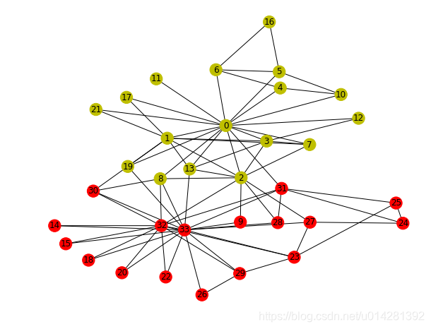
如下图所示，是一个小型社交网络关系图．关系网络中有34个节点，代表34个成员．不同的颜色表示两个不同的(group/community),整个网络中有两个中心节点（０，33)
在这里插入图片描述
:align: center
任务：预测每一个成员，倾向于哪一个（group/community)

用DGL创建一个graph

import dgl

def build_graph():
    g = dgl.DGLGraph()
    # add 34 nodes into the graph; nodes are labeled from 0~33
    g.add_nodes(34)
    # all 78 edges as a list of tuples, tuple(小，大) 
    edge_list = [(1, 0), (2, 0), (2, 1), (3, 0), (3, 1), (3, 2),
        (4, 0), (5, 0), (6, 0), (6, 4), (6, 5), (7, 0), (7, 1),
        (7, 2), (7, 3), (8, 0), (8, 2), (9, 2), (10, 0), (10, 4),
        (10, 5), (11, 0), (12, 0), (12, 3), (13, 0), (13, 1), (13, 2),
        (13, 3), (16, 5), (16, 6), (17, 0), (17, 1), (19, 0), (19, 1),
        (21, 0), (21, 1), (25, 23), (25, 24), (27, 2), (27, 23),
        (27, 24), (28, 2), (29, 23), (29, 26), (30, 1), (30, 8),
        (31, 0), (31, 24), (31, 25), (31, 28), (32, 2), (32, 8),
        (32, 14), (32, 15), (32, 18), (32, 20), (32, 22), (32, 23),
        (32, 29), (32, 30), (32, 31), (33, 8), (33, 9), (33, 13),
        (33, 14), (33, 15), (33, 18), (33, 19), (33, 20), (33, 22),
        (33, 23), (33, 26), (33, 27), (33, 28), (33, 29), (33, 30),
        (33, 31), (33, 32)]
    # zip() 利用 * 号操作符，可以将元组解压为列表。
    src, dst = tuple(zip(*edge_list))
    g.add_edges(src, dst)
    # DGL构建的是一个有向图, (src, dst), (dst, src) 双向
    g.add_edges(dst, src)
    return g

图中节点和边的数量

G = build_graph()
print('We have %d nodes.' % G.number_of_nodes())
print('We have %d edges.' % G.number_of_edges())

We have 34 nodes.
We have 156 edges.

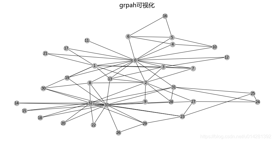
用networkx可视化grpah

import networkx as nx
import matplotlib.pyplot as plt
import matplotlib as mpl
msyh = mpl.font_manager.FontProperties(fname='./msyh.ttf')
%matplotlib inline
# 没有方向的
nx_G = G.to_networkx().to_undirected()
pos = nx.kamada_kawai_layout(nx_G)
plt.figure(figsize=(16, 8))
plt.title('grpah可视化', fontproperties=msyh, fontsize=20)
nx.draw(nx_G, pos, with_labels=True, node_color=[[.7, .7, .7]])

在这里插入图片描述

构造nodes/edges的特征

图神经网络利用图中节点和边特征进行训练，节点要经过one-hot编码，用一个向量来表示，例如：node $v_i$ '经过one-hot编码后的特征向量是： $[0,\ldots,1,\dots,0]$ , $i^{th}$ 即在向量１索引的位置．在DGL中允许我们给节点增加新的特征，在沿着特征向量的第一个axis方向上拼接．

import torch

G.ndata['feat'] = torch.eye(34)


# node 2的特征
print(G.nodes[2].data['feat'])

# node 10 and 11's features
print(G.nodes[[10, 11]].data['feat'])

tensor([[0., 0., 1., 0., 0., 0., 0., 0., 0., 0., 0., 0., 0., 0., 0., 0., 0., 0.,
         0., 0., 0., 0., 0., 0., 0., 0., 0., 0., 0., 0., 0., 0., 0., 0.]])
tensor([[0., 0., 0., 0., 0., 0., 0., 0., 0., 0., 1., 0., 0., 0., 0., 0., 0., 0.,
         0., 0., 0., 0., 0., 0., 0., 0., 0., 0., 0., 0., 0., 0., 0., 0.],
        [0., 0., 0., 0., 0., 0., 0., 0., 0., 0., 0., 1., 0., 0., 0., 0., 0., 0.,
         0., 0., 0., 0., 0., 0., 0., 0., 0., 0., 0., 0., 0., 0., 0., 0.]])

图卷积神经网络 (GCN)- Graph Convolutional Network

使用图卷积神经网络进行分类任务，关于图神经网络更多细节可以参考论文`Kipf and Welling https://arxiv.org/abs/1609.02907＇下图为图卷积网络中的其中一层 $l$ .

在这里插入图片描述

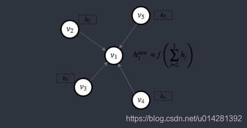
$l$ 层, 每个节点 $v_i^l$ 都有一个one-hot编码的特征向量　 $h_i^l$ .
在GCN中每一层中的每个节点，会聚合与其邻接且指向它的节点的特征向量 $h_i^l$ ,在经过放射变换生成新的特征向量，更新该节点的特征向量．
以上图中的 $v_1^l$ 为例：它利用相邻节点的特征更新自己的特征．(message-passing paradigm)(消息传递范式）
- $h_1^{new} = f(h_2 + h_3 + h_4 + h_5)$

import torch.nn as nn
import torch.nn.functional as F

# Define the message & reduce function
# gcn_message : 返回每个节点携带的message
# gcn_reduce : 通过节点的mailbox收到来自邻接节点的message,计算该节点的new h(feature vector)
# NOTE: we ignore the GCN's normalization

def gcn_message(edges):
    # edges : batch of edges.
    # This computes a (batch of) message called 'msg' using the source node's feature 'h'.
    return {'msg' : edges.src['feat']}

def gcn_reduce(nodes):
    # nodes : batch of nodes.
    # This computes the new 'h' features by summing received 'msg' in each node's mailbox.
    return {'feat' : torch.sum(nodes.mailbox['msg'], dim=1)}

# Define the GCNLayer module
class GCNLayer(nn.Module):
    def __init__(self, in_feats, out_feats):
        super(GCNLayer, self).__init__()
        self.linear = nn.Linear(in_feats, out_feats)

    def forward(self, g, inputs):
        # g : graph , inputs :node features(message)
        # first set the node features
        g.ndata['feat'] = inputs
        # 沿着边发送message
        g.send(g.edges(), gcn_message)
        ## check mailbox,更新自己的meaage即（feature vector)
        g.recv(g.nodes(), gcn_reduce)
        # get the result node features
        h = g.ndata.pop('feat')
        # linear transformation
        return self.linear(h)

# Define a 2-layer GCN model
class GCN(nn.Module):
    def __init__(self, in_feats, hidden_size, num_classes):
        super(GCN, self).__init__()
        self.gcn1 = GCNLayer(in_feats, hidden_size)
        self.gcn2 = GCNLayer(hidden_size, num_classes)

    def forward(self, g, inputs):
        h = self.gcn1(g, inputs)   #　没有显式的调用类GCNLayer的forward()方法
        h = torch.relu(h)
        h = self.gcn2(g, h)
        return h
    
# in_feats : 原始图中节点的数量
# hidden_size : 隐藏层，图中节点的数量
# num_classes : 图中，community的数量
net = GCN(34, 5, 2)

数据的准备和初始化

特征向量的初始化（one-hot编码）
其实这是一个半监督学习，只有地0, 33个成员有明确的label.

inputs = torch.eye(34)    # nodes特征向量初始化，即one-hot编码
labeled_nodes = torch.tensor([0, 33])  # labeled_nodes, 两个community中中心节点０，３３
labels = torch.tensor([0, 1])  # ０，１ 表示两个不同的群体

training

optimizer = torch.optim.Adam(net.parameters(), lr=0.01)
all_logits = []
train_loss = []
for epoch in range(50):
    logits = net(G, inputs)
    # 保存中间结果用于可视化
    all_logits.append(logits.detach())
    logp = F.log_softmax(logits, 1)
    # we only compute loss for labeled nodes
    loss = F.nll_loss(logp[labeled_nodes], labels)
    train_loss.append(loss.item())
    optimizer.zero_grad()
    loss.backward()
    optimizer.step()
    if epoch%10 == 0:
        print('Epoch %d | Loss: %.4f' % (epoch+10, loss.item()))

Epoch 10 | Loss: 1.0756
Epoch 20 | Loss: 0.2680
Epoch 30 | Loss: 0.0105
Epoch 40 | Loss: 0.0007
Epoch 50 | Loss: 0.0002

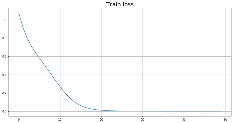
plt.figure(figsize=(14, 7))
plt.plot(train_loss)
plt.title('Train loss',fontsize=20)
plt.grid()

在这里插入图片描述

init_features and new_features

original_features = inputs.detach().numpy()
now_features = logits.detach().numpy()
print('original input shape :',original_features.shape)
print('now_features shape :',now_features.shape)

original input shape : (34, 34)
now_features shape : (34, 2)

original_features

array([[1., 0., 0., ..., 0., 0., 0.],
       [0., 1., 0., ..., 0., 0., 0.],
       [0., 0., 1., ..., 0., 0., 0.],
       ...,
       [0., 0., 0., ..., 1., 0., 0.],
       [0., 0., 0., ..., 0., 1., 0.],
       [0., 0., 0., ..., 0., 0., 1.]], dtype=float32)

now_features

array([[ 5.637299  , -3.288989  ],
       [ 4.512527  , -1.8517829 ],
       [ 4.158336  ,  2.1036315 ],
       [ 4.244565  , -3.1265435 ],
       [ 2.0464027 , -2.2225604 ],
       [ 2.312477  , -2.3433352 ],
       [ 2.2144208 , -2.490665  ],
       [ 3.8895829 , -3.0338702 ],
       [ 3.1264923 ,  2.0993629 ],
       [ 1.4217453 ,  0.24895817],
       [ 1.9483465 , -2.3698897 ],
       [ 1.3896602 , -1.5943918 ],
       [ 2.007552  , -1.8470225 ],
       [ 4.3145075 , -1.6916609 ],
       [ 0.5206586 ,  2.8570418 ],
       [ 0.5206586 ,  2.8570418 ],
       [ 0.7254505 , -1.423414  ],
       [ 2.2787623 , -2.311398  ],
       [ 0.5206586 ,  2.8570418 ],
       [ 2.7036874 , -0.9691887 ],
       [ 0.5206586 ,  2.8570418 ],
       [ 2.2787623 , -2.311398  ],
       [ 0.5206586 ,  2.8570418 ],
       [ 0.759069  ,  5.7162037 ],
       [ 0.24731699,  1.3865811 ],
       [ 0.3594055 ,  0.51410866],
       [ 0.5375926 ,  1.8520871 ],
       [ 1.6634679 ,  1.1023602 ],
       [ 1.5355374 ,  0.53307414],
       [ 0.6524333 ,  4.1704736 ],
       [ 1.5976448 ,  2.5490031 ],
       [ 2.212409  ,  3.619369  ],
       [ 2.5465662 ,  6.8266993 ],
       [ 2.0438857 , 11.185618  ]], dtype=float32)

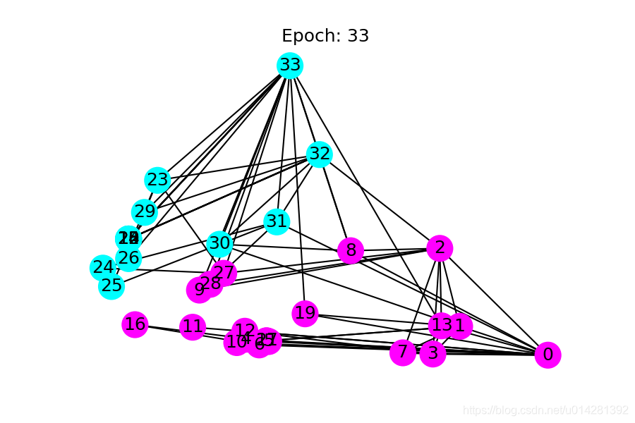
训练过程的可视化

import matplotlib.animation as animation
import matplotlib.pyplot as plt
import pandas as pd
from IPython.display import HTML
import warnings
warnings.filterwarnings('ignore')
%matplotlib notebook
# 2维空间中的位置变化
def plot_scatter(i):
    pos = all_logits[i]
    plt.scatter(pos[:,0], pos[:,1],s=10)

# 图网络可视化
def draw(i):
    cls1color = '#00FFFF'
    cls2color = '#FF00FF'
    pos = {}
    colors = []
    for v in range(34):
        pos[v] = all_logits[i][v].numpy()
        cls = pos[v].argmax()
        colors.append(cls1color if cls else cls2color)
    ax.cla()
    ax.axis('off')
    ax.set_title('Epoch: %d' % i)
    nx.draw_networkx(nx_G.to_undirected(), pos, node_color=colors,
            with_labels=True, node_size=300, ax=ax)

fig = plt.figure(dpi=100)
ani_1 = animation.FuncAnimation(fig, draw, frames=len(all_logits), interval=200)
HTML(ani.to_jshtml())

这是一张截图：
在这里插入图片描述

图神经网络初探：build a simple graph nets

Building a simple graph nets model : (for classification)

问题描述：

用DGL创建一个graph

构造nodes/edges的特征

图卷积神经网络 (GCN)- Graph Convolutional Network

数据的准备和初始化

training

init_features and new_features

训练过程的可视化

猜你喜欢