线性回归---with multiple variables（Octave转换为Python)

详细代码可参考：github

多变量线性回归

实例：
已知房屋面积和卧室数量，预测房价 计算公式：Price = theta0*1 + theta1*square + theta2*num_houses

1.特征归一化

房间面积和卧室数量相差有2-3个数量级，如果直接利用梯度下降来计算的话，房屋面积可以让函数更快收敛，因此将两个特征进行归一化。

归一化公式：

参考代码：

def featureNormalize(self):
	mu = np.mean(self.x, axis=0)
	sigma = np.std(self.x, axis=0, ddof=1)  # 注意ddof参数，必须是1
	self.x_norm = (self.x - mu)/sigma
	self.x = np.hstack([np.ones((47, 1)), self.x_norm])

注意：每个特征都是一列，因此操作多是在列的基础上操作，参数axis=0, 同时注意np.std的使用，ddof参数尤其需要注意。

2. 梯度下降法计算theta

设置步长alpha = 0.01，迭代次数400次，此次损失函数使用向量形式表示：

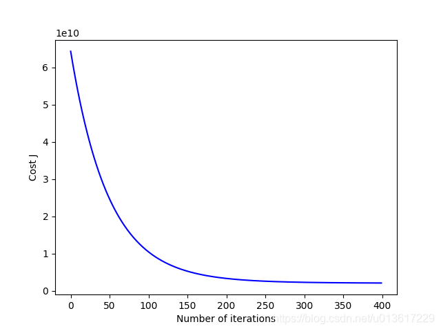
在步长0.01的情况下，损失函数J的曲线，如下图所示。

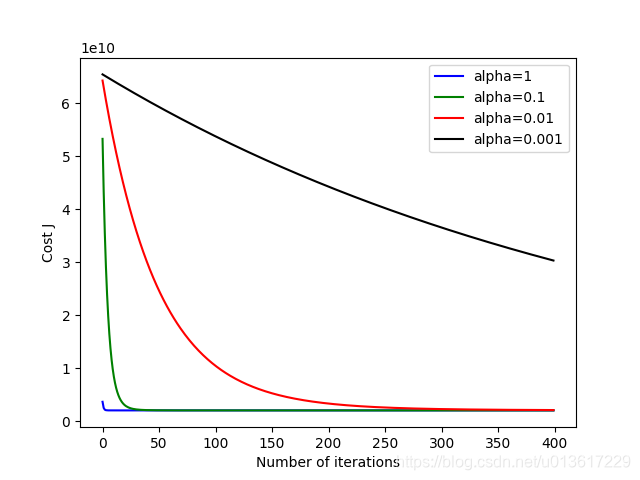
同时设置alpha = 0.001、0.01、0.1、1，见对比图，可以清晰的看出当alpha较大的时候，迅速收敛，而当alpha太小的时候，收敛速度又太慢，可以看出设置alpha=0.01最好。

参考代码：

def gradientDescentMulti(self):
	m = len(self.y)
	self.J_history = np.zeros((self.iters, 1))

	for i in range(self.iters):
		self.theta = self.theta-self.alpha/m*np.dot((np.dot(self.x, self.theta)-self.y).transpose(), self.x).transpose()
		self.J_history[i] = self.computeCostMulti()
	return self.theta

def convergenceGraph(self):
	plt.plot([x for x in range(400)], self.J_history, 'b')
	plt.xlabel('Number of iterations')
	plt.ylabel('Cost J')
	plt.show()

3.Normal Equations

线性回归中theta的计算也可以不使用梯度下降迭代来计算，使用Normal Equations，公式：

参考代码：

def normalEquations(self):
	self.x = np.hstack([np.ones((47, 1)), self.x])
	self.theta = np.dot(np.dot(np.mat(np.dot(self.x.T, self.x)).I, self.x.T), self.y)
	print(self.theta)