1.导入运行库
from keras.datasets import mnist
from keras.utils import np_utils
import numpy as np
np.random.seed(10)
2.进行数据预处理
(x_Train, y_Train), (x_Test, y_Test) = mnist.load_data()

x_Train4D=x_Train.reshape(x_Train.shape[0],28,28,1).astype('float32')
x_Test4D=x_Test.reshape(x_Test.shape[0],28,28,1).astype('float32')

x_Train4D_normalize = x_Train4D / 255
x_Test4D_normalize = x_Test4D / 255

y_TrainOneHot = np_utils.to_categorical(y_Train)
y_TestOneHot = np_utils.to_categorical(y_Test)
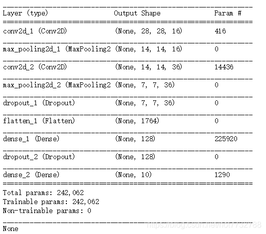
3.建立模型
from keras.models import Sequential
from keras.layers import Dense,Dropout,Flatten,Conv2D,MaxPooling2D
model = Sequential()
model.add(Conv2D(filters=16,
kernel_size=(5,5),
padding='same',
input_shape=(28,28,1),
activation='relu'))
model.add(MaxPooling2D(pool_size=(2, 2)))
model.add(Conv2D(filters=36,
kernel_size=(5,5),
padding='same',
activation='relu'))
model.add(MaxPooling2D(pool_size=(2, 2)))
model.add(Dropout(0.25))
model.add(Flatten())
model.add(Dense(128, activation='relu'))
model.add(Dropout(0.5))
model.add(Dense(10,activation='softmax'))
print(model.summary())
4.训练模型
model.compile(loss='categorical_crossentropy',
optimizer='adam',metrics=['accuracy'])
train_history=model.fit(x=x_Train4D_normalize,
y=y_TrainOneHot,validation_split=0.2,
epochs=20, batch_size=300,verbose=2)
import matplotlib.pyplot as plt
def show_train_history(train_acc,test_acc):
plt.plot(train_history.history[train_acc])
plt.plot(train_history.history[test_acc])
plt.title('Train History')
plt.ylabel('Accuracy')
plt.xlabel('Epoch')
plt.legend(['train', 'test'], loc='upper left')
plt.show()
show_train_history('acc','val_acc')
show_train_history('loss','val_loss')
5.进行模型准确率评估
scores = model.evaluate(x_Test4D_normalize , y_TestOneHot)
scores[1]
6.预测结果
import matplotlib.pyplot as plt
def plot_images_labels_prediction(images,labels,prediction,idx,num=10):
    fig = plt.gcf()
    fig.set_size_inches(12, 14)
    if num>25: num=25
    for i in range(0, num):
        ax=plt.subplot(5,5, 1+i)
        ax.imshow(images[idx], cmap='binary')

        ax.set_title("label=" +str(labels[idx])+
                     ",predict="+str(prediction[idx])
                     ,fontsize=10)

        ax.set_xticks([]);ax.set_yticks([])
        idx+=1
    plt.show()
plot_images_labels_prediction(x_Test,y_Test,prediction,idx=0)
import pandas as pd
pd.crosstab(y_Test,prediction,
            rownames=['label'],colnames=['predict'])
df = pd.DataFrame({'label':y_Test, 'predict':prediction})