游戏的全过程可以理解为AI智能体和环境之间的互动,我们把其中复杂的因素抽象为三个变量——报酬、行动、状态。
状态(s)
| 编号 | 名称 | 最小值 | 最大值 |
|---|---|---|---|
| 0 | 小车的位置 | -2.4 | 2.4 |
| 1 | 小车的速度 | -inf | inf |
| 2 | 木棒的角度 | -41.8 | 41.8 |
| 3 | 木棒的速度 | -inf | inf |
行动(a)
对于某一个状态s采取的行动A(s)应该包括以下两种:
0: 小车向左移动
1: 小车向右移动
报酬®
木棒每保持平衡1个时间步,就得到1分
每一场游戏的最高得分200分
每一场游戏的结束条件:木棒倾斜角度大于41.8度或者已经到达200分
最终获胜的条件为:最近100场游戏的平均得分高于195
首先基于Q-Learning的方法实现,并解析代码中的一些内容。后面使用DQN的方式来实现
Q-Learning代码实现
import gym
import numpy as np

env = gym.make('CartPole-v0')

max_number_of_steps = 200   # 每一场游戏的最高得分
# 获胜的条件是最近100场平均得分高于195
goal_average_steps = 195
num_consecutive_iterations = 100
num_episodes = 5000
# num_episodes = 1
# 只存储最近100场的得分(可以理解为是一个容量为100的栈)
last_time_steps = np.zeros(num_consecutive_iterations)

# q_table是一个256*2的二维数组
# 离散化后的状态共有4^4=256种可能的取值,每种状态对应一个行动
# q_table[s][a]就是当状态为s时做出行动a的有利程度评价值
# 我们的AI模型要训练学习的就是这个映射关系表
q_table = np.random.uniform(low=-1, high=1, size=(4 ** 4, env.action_space.n))

# np.linspace() 等差数列
# 分箱处理函数,把[clip_min, clip_max]区间平均分为num段,位于i段区间的特征值x会被离散化为i
def bins(clip_min, clip_max, num):
#    print(np.linspace(clip_min, clip_max, num + 1))
    return np.linspace(clip_min, clip_max, num + 1)[1:-1]

# 离散化处理,将由4个连续特征值组成的状态矢量转换为一个0~~255的整数离散值
def digitize_state(observation):
	# 将矢量打散回4个连续特征值
    cart_pos, cart_v, pole_angle, pole_v = observation
#    print(cart_pos)
#    print(np.digitize(cart_pos, bins=bins(-2.4, 2.4, 4)))
	# 分别对各个连续特征值进行离散化(分箱处理)
    digitized = [np.digitize(cart_pos, bins=bins(-2.4, 2.4, 4)),
                 np.digitize(cart_v, bins=bins(-3.0, 3.0, 4)),
                 np.digitize(pole_angle, bins=bins(-0.5, 0.5, 4)),
                 np.digitize(pole_v, bins=bins(-2.0, 2.0, 4))]
#    print(digitized)
#    for i, x in enumerate(digitized):
#        print(i, x)
#        print(x)

#    print(sum([x * (4 ** i) for i, x in enumerate(digitized)]))
	# 将4个离散值再组合为一个离散值,作为最终结果
    return sum([x * (4 ** i) for i, x in enumerate(digitized)])

# 根据本次的行动及其反馈(下一个时间步的状态),返回下一次的最佳行动
def get_action(state, action, observation, reward, episode):
    next_state = digitize_state(observation) # 获取下一个时间步的状态,并将其离散化
    epsilon = 0.5 * (0.99 ** episode) # ع-贪心策略
    if epsilon <= np.random.uniform(0, 1):
        next_action = np.argmax(q_table[next_state])
    else:
        next_action = np.random.choice([0,1])

    alpha = 0.2    # 学习系数
    gamma = 0.99   # 报酬衰减系数
    q_table[state, action] = (1 - alpha) * q_table[state, action] + alpha * (reward + gamma * q_table[next_state, next_action])
    # -------------------------------------------------------------------------------------------
    return next_action, next_state

for episode in range(num_episodes):
    observation = env.reset()   # 初始化本场游戏的环境
    state = digitize_state(observation)     # 获取初始状态值
#    print(state)
#    print(q_table)
#    print(q_table[state])
    action = np.argmax(q_table[state])  # 根据状态值做出行动决策
#    print(action)
    episode_reward = 0

    # 一场游戏分为一个个时间步
    for t in range(max_number_of_steps):
        env.render()  # 更新并渲染游戏画面
        observation, reward, done, info = env.step(action)  # 获取本次行动的反馈结果
        # 对致命错误行动进行极大力度的惩罚,让模型狠狠地吸取教训
        if done:
            print('kill!!!')
            reward = -200

        action, state = get_action(state, action, observation, reward, episode)
        episode_reward += reward
        if done:
            print('%d Episode finished after %f time steps / mean %f' % (episode, t + 1, last_time_steps.mean()))
            last_time_steps = np.hstack((last_time_steps[1:], [episode_reward]))
            break

        if (last_time_steps.mean() >= goal_average_steps):
            print('Episode %d train agent successfuly!' % episode)
            break

print('Failed!')
env.close()
这里代码中添加了很多的print打印信息的代码。是为了刚开始理解某些代码的实现,也为了防止以后再看时,一时不知道何意。
下面就离散化处理做出解析:
def bins():
print np.linspace(clip_min, clip_max, num+1)
等差数列,输出结果为:
[-2.4, -1.2, 0, 1.2, 2.4]
[-3, -1.5, 0, 1.5, 3]
[-0.5, -0.25, 0, 0.25, 0.5]
[-2, -1, 0, 1, 2]
而函数bins()中输出的结果去除了第一个和最后一个数
print np.linspace(clip_min, clip_max, num+1) [1,-1]
结果为:
[-1.2, 0, 1.2]
[-1.5, 0, 1.5]
[-0.25, 0, 0,25]
[-1, 0, 1]
分箱处理
:(digitized)分别对各个连续特征值进行离散化
digitize(data, bins)
digitize()函数是numpy的一个内置函数。
下面举例说明:
import random as rd
data = [rd.randint(a=100, b=1000) for _ in range(20)]
bins = [ 200, 300, 400, 500, 600, 700, 800, 900, 1000]
print('data:', data)
print('bins:', bins)
print('np.digitize(data,bins):', np.digitize(data, bins))
运行结果如下:

Tips:digitize(data, bins)函数对data列表似乎没有什么要求,但是对bins列表是有要求的。
要求bins汇总的数据要么是升序的,要么是将序的,不能是随意的一堆数。
digitize(data, bins)函数执行的过程大概如下:
相当于两层for循环。
首先最外面的一层:顺序的遍历data列表,取出当前的一个数a,然后顺序的遍历bins列表,返回bins列表中某个数的索引,如何找呢?规则如下:如果bins列表是升序的,那么如果满足bins[i-1]<=a<bins[i],那么就保存i,然后回到外层循环继续上面的操作,如果bins列表是降序的,那么如果满足bins[i]<=a<bins[i-1],那么就保存i,当data列表遍历完之后,就返回由i组成的来源于bins的索引的一个索引列表。
解析CartPole中离散化的处理方式
某一时刻,环境的状态:
cart_pos, cart_v, pole_angle, pole_v = observation
分别对各个连续特征值进行离散化(分箱处理):
digitized = [np.digitize(cart_pos, bins=bins(-2.4, 2.4, 4)),
                     np.digitize(cart_v, bins=bins(-3.0, 3.0, 4)),
                     np.digitize(pole_angle, bins=bins(-0.5, 0.5, 4)),
                     np.digitize(pole_v, bins=bins(-2.0, 2.0, 4))]
假设这个时刻observation的值为 (-1.4, 1.2, 0.27, -0.3)
即:cart_pos = -1.4, cart_v = 1.2, pole_angle = 0.24, pole_v = -0.3
cart_pos : -1.4<-1.2 故np.digitize(cart_pos, bins=bins(-2.4, 2.4, 4)) = 0
同理:
cart_v:0<1.2<1.5 np.digitize(cart_v, bins=bins(-3.0, 3.0, 4)) = 2
pole_angle:0<0.27<0.25 np.digitize(pole_angle, bins=bins(-0.5, 0.5,4)) = 3
pole_v:-1<-0.3<0 np.digitize(pole_v, bins=bins(-2.0, 2.0, 4)) = 1
则digitized的值为:[0, 2, 3, 1]
将4个离散值再组合为一个离散值,作为最终结果
return sum([x * (4 ** i) for i, x in enumerate(digitized)])
这里 :
i = 0, x = 0
i = 1, x = 2
i = 2, x = 3
i = 3, x = 1
结果为:0x4^0 + 1x4^2 + 2x4^3 + 3x4^1 = 0 + 16 + 128 + 12 = 156
该环境就是通过把环境的状态离散化为256个值(0~255)来处理
Gym简介
观测(observations)
env.step()函数来对每一步进行仿真,在Gym中,env.step()会返回4个参数
观测 Observation(Object):当前step执行后,环境的观测(类型为对象)。例如,从相机获取的像素点,机器人各个关节的角度或棋盘游戏当前的状态。
奖励 Reward(Float):执行上一步动作(action)后,智能体(agent)获得的奖励(浮点类型),不同的环境中奖励值变化范围也有不同,但是强化学习的目标就是总奖励值最大。
完成 Done(Boolen):表示是否需要将环境重置env.reset,大多数情况下,当Done为True时,就表明当前回合(episode)或者实验(tial)结束。例如当机器人摔倒或者掉出台面,就应当终止当前回合进行重置(reset)。
信息 Info(Dict):针对调试过程的诊断信息,在标准的智能体仿真评估当中不会使用到这个info
空间(spaces)
每次执行的动作(action)都是从环境动作空间中随机进行选取的,但是这些动作(action)是什么?在Gym的仿真环境中,有运动空间action_space和观测空间observation_space两个指标,程序中被定义为Space类型,用于描述有效的运动和观测的格式和范围。
action_space是一个离散Discrete类型,从discrete.py中可知,范围是一个{0,1,…,n-1}长度的非负正数集合。
observation_space是一个Box类型。(state)
实例:
print(env.action_space)
print(env.observation_space)
print(env.observation_space.high)
print(env.observation_space.low)
# Discrete(2)
# Box(4,)
# [  4.80000019e+00   3.40282347e+38   4.18879032e-01   3.40282347e+38]
# [ -4.80000019e+00  -3.40282347e+38  -4.18879032e-01  -3.40282347e+38]
这个是CartPole-v0的实例,action_space有两个动作(向左移动,向右移动),而状态空间有4个值。
DQN代码实现
run_PartPole.py
import gym
from RL_brain import DeepQNetwork

import os
os.environ["CUDA_DEVICE_ORDER"] = "PCI_BUS_ID"
os.environ['CUDA_VISIBLE_DEVICES'] = "0"

env = gym.make('CartPole-v0')
env = env.unwrapped

print(env.action_space)
print(env.observation_space)
print(env.observation_space.high)
print(env.observation_space.low)
# Discrete(2)
# Box(4,)
# [  4.80000019e+00   3.40282347e+38   4.18879032e-01   3.40282347e+38]
# [ -4.80000019e+00  -3.40282347e+38  -4.18879032e-01  -3.40282347e+38]

RL = DeepQNetwork(n_actions=env.action_space.n,
                  n_features=env.observation_space.shape[0],
                  learning_rate=0.01, e_greedy=0.9,
                  replace_target_iter=100, memory_size=2000,
                  e_greedy_increment=0.001,)

total_steps = 0


for i_episode in range(5000):
    print(i_episode)

    observation = env.reset()
    ep_r = 0
    i = 0
    while True:
        env.render()

        action = RL.choose_action(observation)

        observation_, reward, done, info = env.step(action)

        # the smaller theta and closer to center the better
        x, x_dot, theta, theta_dot = observation_
        r1 = (env.x_threshold - abs(x))/env.x_threshold - 0.8
        r2 = (env.theta_threshold_radians - abs(theta))/env.theta_threshold_radians - 0.5
        reward = r1 + r2

        RL.store_transition(observation, action, reward, observation_)

        ep_r += reward
        if total_steps > 1000:
            RL.learn()

        i += 1
        if done:

            print('episode: ', i_episode,
                  'ep_r: ', round(ep_r, 2),
                  ' epsilon: ', round(RL.epsilon, 2))
            break

        observation = observation_
        total_steps += 1

RL.plot_cost()
RL_brain.py
import numpy as np
import pandas as pd
import tensorflow as tf


# Deep Q Network off-policy
class DeepQNetwork:
    def __init__(
            self,
            n_actions,
            n_features,
            learning_rate=0.01,
            reward_decay=0.9,
            e_greedy=0.9,
            replace_target_iter=300,
            memory_size=500,
            batch_size=32,
            e_greedy_increment=None,
            output_graph=False,
    ):
        self.n_actions = n_actions
        self.n_features = n_features
        self.lr = learning_rate
        self.gamma = reward_decay
        self.epsilon_max = e_greedy
        self.replace_target_iter = replace_target_iter
        self.memory_size = memory_size
        self.batch_size = batch_size
        self.epsilon_increment = e_greedy_increment
        self.epsilon = 0 if e_greedy_increment is not None else self.epsilon_max

        # total learning step
        self.learn_step_counter = 0

        # initialize zero memory [s, a, r, s_]
        self.memory = np.zeros((self.memory_size, n_features * 2 + 2))

        # consist of [target_net, evaluate_net]
        self._build_net()
        t_params = tf.get_collection('target_net_params')
        e_params = tf.get_collection('eval_net_params')
        self.replace_target_op = [tf.assign(t, e) for t, e in zip(t_params, e_params)]

        self.sess = tf.Session()

        if output_graph:
            # $ tensorboard --logdir=logs
            # tf.train.SummaryWriter soon be deprecated, use following
            tf.summary.FileWriter("logs/", self.sess.graph)

        self.sess.run(tf.global_variables_initializer())
        self.cost_his = []

    def _build_net(self):
        # ------------------ build evaluate_net ------------------
        self.s = tf.placeholder(tf.float32, [None, self.n_features], name='s')  # input
        self.q_target = tf.placeholder(tf.float32, [None, self.n_actions], name='Q_target')  # for calculating loss
        with tf.variable_scope('eval_net'):
            # c_names(collections_names) are the collections to store variables
            c_names, n_l1, w_initializer, b_initializer = \
                ['eval_net_params', tf.GraphKeys.GLOBAL_VARIABLES], 10, \
                tf.random_normal_initializer(0., 0.3), tf.constant_initializer(0.1)  # config of layers

            # first layer. collections is used later when assign to target net
            with tf.variable_scope('l1'):
                w1 = tf.get_variable('w1', [self.n_features, n_l1], initializer=w_initializer, collections=c_names)
                b1 = tf.get_variable('b1', [1, n_l1], initializer=b_initializer, collections=c_names)
                l1 = tf.nn.relu(tf.matmul(self.s, w1) + b1)

            # second layer. collections is used later when assign to target net
            with tf.variable_scope('l2'):
                w2 = tf.get_variable('w2', [n_l1, self.n_actions], initializer=w_initializer, collections=c_names)
                b2 = tf.get_variable('b2', [1, self.n_actions], initializer=b_initializer, collections=c_names)
                self.q_eval = tf.matmul(l1, w2) + b2

        with tf.variable_scope('loss'):
            self.loss = tf.reduce_mean(tf.squared_difference(self.q_target, self.q_eval))
        with tf.variable_scope('train'):
            self._train_op = tf.train.RMSPropOptimizer(self.lr).minimize(self.loss)

        # ------------------ build target_net ------------------
        self.s_ = tf.placeholder(tf.float32, [None, self.n_features], name='s_')    # input
        with tf.variable_scope('target_net'):
            # c_names(collections_names) are the collections to store variables
            c_names = ['target_net_params', tf.GraphKeys.GLOBAL_VARIABLES]

            # first layer. collections is used later when assign to target net
            with tf.variable_scope('l1'):
                w1 = tf.get_variable('w1', [self.n_features, n_l1], initializer=w_initializer, collections=c_names)
                b1 = tf.get_variable('b1', [1, n_l1], initializer=b_initializer, collections=c_names)
                l1 = tf.nn.relu(tf.matmul(self.s_, w1) + b1)

            # second layer. collections is used later when assign to target net
            with tf.variable_scope('l2'):
                w2 = tf.get_variable('w2', [n_l1, self.n_actions], initializer=w_initializer, collections=c_names)
                b2 = tf.get_variable('b2', [1, self.n_actions], initializer=b_initializer, collections=c_names)
                self.q_next = tf.matmul(l1, w2) + b2

    def store_transition(self, s, a, r, s_):
        if not hasattr(self, 'memory_counter'):
            self.memory_counter = 0

        transition = np.hstack((s, [a, r], s_))

        # replace the old memory with new memory
        index = self.memory_counter % self.memory_size
        self.memory[index, :] = transition

        self.memory_counter += 1

    def choose_action(self, observation):
        # to have batch dimension when feed into tf placeholder
        observation = observation[np.newaxis, :]

        if np.random.uniform() < self.epsilon:
            # forward feed the observation and get q value for every actions
            actions_value = self.sess.run(self.q_eval, feed_dict={self.s: observation})
            action = np.argmax(actions_value)
        else:
            action = np.random.randint(0, self.n_actions)
        return action

    def learn(self):
        # check to replace target parameters
        if self.learn_step_counter % self.replace_target_iter == 0:
            self.sess.run(self.replace_target_op)
            print('\ntarget_params_replaced\n')

        # sample batch memory from all memory
        if self.memory_counter > self.memory_size:
            sample_index = np.random.choice(self.memory_size, size=self.batch_size)
        else:
            sample_index = np.random.choice(self.memory_counter, size=self.batch_size)
        batch_memory = self.memory[sample_index, :]

        q_next, q_eval = self.sess.run(
            [self.q_next, self.q_eval],
            feed_dict={
                self.s_: batch_memory[:, -self.n_features:],  # fixed params
                self.s: batch_memory[:, :self.n_features],  # newest params
            })

        # change q_target w.r.t q_eval's action
        q_target = q_eval.copy()

        batch_index = np.arange(self.batch_size, dtype=np.int32)
        eval_act_index = batch_memory[:, self.n_features].astype(int)
        reward = batch_memory[:, self.n_features + 1]

        q_target[batch_index, eval_act_index] = reward + self.gamma * np.max(q_next, axis=1)

        """
        For example in this batch I have 2 samples and 3 actions:
        q_eval =
        [[1, 2, 3],
         [4, 5, 6]]

        q_target = q_eval =
        [[1, 2, 3],
         [4, 5, 6]]

        Then change q_target with the real q_target value w.r.t the q_eval's action.
        For example in:
            sample 0, I took action 0, and the max q_target value is -1;
            sample 1, I took action 2, and the max q_target value is -2:
        q_target =
        [[-1, 2, 3],
         [4, 5, -2]]

        So the (q_target - q_eval) becomes:
        [[(-1)-(1), 0, 0],
         [0, 0, (-2)-(6)]]

        We then backpropagate this error w.r.t the corresponding action to network,
        leave other action as error=0 cause we didn't choose it.
        """

        # train eval network
        _, self.cost = self.sess.run([self._train_op, self.loss],
                                     feed_dict={self.s: batch_memory[:, :self.n_features],
                                                self.q_target: q_target})
        self.cost_his.append(self.cost)

        # increasing epsilon
        self.epsilon = self.epsilon + self.epsilon_increment if self.epsilon < self.epsilon_max else self.epsilon_max
        self.learn_step_counter += 1

    def plot_cost(self):
        import matplotlib.pyplot as plt
        plt.plot(np.arange(len(self.cost_his)), self.cost_his)
        plt.ylabel('Cost')
        plt.xlabel('training steps')
        plt.show()
代码解析:
两个策略:
记忆库
暂时冻结q_target(切断相关性)
网络结构
分为两个网络:eval_net, target_net
两个网络的结构一样,结构为
输入数据s:[batch_size, n_features] = [32, 4]
w1:[n_feature, n_l1] = [4, 10]
b1:[1, n_l1] = [1, 10]
l1 = tf.nn.relu(tf.matmul(s, w1) + b1)
w2:[n_l1, n_actions] = [10, 2]
b2:[1, n_actions] = [1, 2]
q_eval/q_next = tf.matmul(l1, w2) + b2
记忆库
def store_transition(sefl, s, a, r, s_)
记忆库存储的内容
self.memory = np.zeros((self.memory_size, n_features * 2 + 2))
((500, 10))
存储500个记录, 每个记录中10个元素
每个元素分别为:当前状态(4个),该状态执行的动作(1个),reward(1个),下一个状态(4个)
Learn
1、首先产生500内32个随机数,作为从记忆库中选取记录的索引值。
2、使用从记忆库中获得的记录,经过eval_net和target_net得到q_next, q_eval
q_next, q_eval = self.sess.run(
            [self.q_next, self.q_eval],
            feed_dict={
                self.s_: batch_memory[:, -self.n_features:],  # fixed params
                self.s: batch_memory[:, :self.n_features],  # newest params
            })
下面是DQN的Loss函数
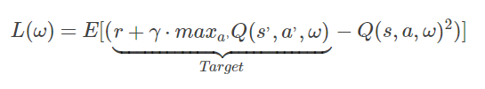
3、我们这里要先得到Target(目标值)
当前状态为上面获取的32个记录中的s,上面得到了q_next, q_eval
先假设q_target = q_eval.copy(),使用历史数据,就是记忆库中的记录来求Target
从Loss函数中可以看到,Target = r + gamma * maxQ(s’, a’, w)
其实就是设置Target中的数值,而q_target的数据格式为 (batch_size, n_action) = (32, 2)
所以在当前状态下,这里只需要赋值,执行动作的那个Q值
4、下一步,从记录中获取当前状态下,执行那个动作和执行该动作后获得的reward
batch_index = np.arange(self.batch_size, dtype=np.int32) # incex
        eval_act_index = batch_memory[:, self.n_features].astype(int) # action
    #    print('@@@@@@@@@@@@@@@@@@@@@@@@')
    #    print(batch_memory[:, self.n_features])
    #    print(eval_act_index)
        reward = batch_memory[:, self.n_features + 1] # reward
该处代码输出的内容
@@@@@@@@@@@@@@@@@@@@@@@@
[ 1. 0. 1. 0. 0. 0. 0. 1. 0. 0. 0. 0. 0. 0. 0. 0. 1. 0.
0. 0. 1. 1. 1. 1. 0. 1. 0. 0. 0. 1. 0. 0.]
[1 0 1 0 0 0 0 1 0 0 0 0 0 0 0 0 1 0 0 0 1 1 1 1 0 1 0 0 0 1 0 0]
q_target[batch_index, eval_act_index] = reward + self.gamma * np.max(q_next, axis=1)
5、train eval network
# train eval network
        _, self.cost = self.sess.run([self._train_op, self.loss],
                                     feed_dict={self.s: batch_memory[:, :self.n_features],
                                                self.q_target: q_target})
训练更新eval中的参数值,然后每训练300次更新target net中的参数值
参考:
https://blog.csdn.net/gg_18826075157/article/details/78163386
莫烦大神视频及代码实例