0.导航
| 这个作业属于哪个课程 |
人工智能实战 |
| 这个作业的要求在哪里 |
人工智能实战第五次作业(个人) |
| 我在这个课程的目标是 |
开拓视野,积累AI实战经验 |
| 这个作业在哪个具体方面帮助我 |
了解sigmoid激活函数和交叉熵函损失数,掌握用二分类的思想实现逻辑与门和或门的方法 |
1.具体作业内容
2.过程及代码
| x1 |
0 |
0 |
1 |
1 |
| x2 |
0 |
1 |
0 |
1 |
| y |
0 |
0 |
0 |
1 |
| x1 |
0 |
0 |
1 |
1 |
| x2 |
0 |
1 |
0 |
1 |
| y |
0 |
1 |
1 |
1 |
import numpy as np
import matplotlib.pyplot as plt

# 设置逻辑与门的样本和标签数据
def Read_AND_Data():
    X = np.array([0,0,1,1,0,1,0,1]).reshape(2,4)
    Y = np.array([0,0,0,1]).reshape(1,4)
    return X,Y

# 设置逻辑或门的样本和标签数据
def Read_OR_Data():
    X = np.array([0,0,1,1,0,1,0,1]).reshape(2,4)
    Y = np.array([0,1,1,1]).reshape(1,4)
    return X,Y

# Sigmoid函数
def Sigmoid(x):
    s=1/(1+np.exp(-x))
    return s

# 前向计算
def ForwardCalculationBatch(W, B, batch_X):
    Z = np.dot(W, batch_X) + B
    A = Sigmoid(Z)
    return A

# 反向计算
def BackPropagationBatch(batch_X, batch_Y, A):
    m = batch_X.shape[1]
    dZ = A - batch_Y
    dB = dZ.sum(axis=1, keepdims=True)/m
    dW = np.dot(dZ, batch_X.T)/m
    return dW, dB

# 更新权重参数
def UpdateWeights(W, B, dW, dB, eta):
    W = W - eta * dW
    B = B - eta * dB
    return W, B

# 计算损失函数
def CheckLoss(W, B, X, Y):
    m = X.shape[1]
    A = ForwardCalculationBatch(W, B, X)
    # Cross Entropy
    J = np.sum(-(np.multiply(Y, np.log(A)) + np.multiply(1 - Y, np.log(1 - A))))
    loss = J / m
    return loss

# 初始化权重值
def InitialWeights(num_input, num_output, method):
    if method == "zero":
        # zero
        W = np.zeros((num_output, num_input))
    elif method == "norm":
        # normalize
        W = np.random.normal(size=(num_output, num_input))
    elif method == "xavier":
        # xavier
        W=np.random.uniform(
            -np.sqrt(6/(num_input+num_output)),
            np.sqrt(6/(num_input+num_output)),
            size=(num_output,num_input))

    B = np.zeros((num_output, 1))
    return W,B

# 这里直接搬教案代码了
def train(X, Y, ForwardCalculationBatch, CheckLoss):
    num_example = X.shape[1]
    num_feature = X.shape[0]
    num_category = Y.shape[0]
    # hyper parameters
    eta = 0.5
    max_epoch = 10000
    # W(num_category, num_feature), B(num_category, 1)
    W, B = InitialWeights(num_feature, num_category, "zero")
    # calculate loss to decide the stop condition
    loss = 5        # initialize loss (larger than 0)
    error = 2e-3    # stop condition

    # if num_example=200, batch_size=10, then iteration=200/10=20
    for epoch in range(max_epoch):
        for i in range(num_example):
            # get x and y value for one sample
            x = X[:,i].reshape(num_feature,1)
            y = Y[:,i].reshape(1,1)
            # get z from x,y
            batch_a = ForwardCalculationBatch(W, B, x)
            # calculate gradient of w and b
            dW, dB = BackPropagationBatch(x, y, batch_a)
            # update w,b
            W, B = UpdateWeights(W, B, dW, dB, eta)
            # end if
        # end for
        # calculate loss for this batch
        loss = CheckLoss(W,B,X,Y)
        print(epoch,i,loss,W,B)
        # end if
        if loss < error:
            break
    # end for

    return W,B, epoch, loss

# 结果可视化
def ShowResult(W,B,X,Y,title):
    # 根据w, b的值画出分割线
    w = -W[0,0]/W[0,1]
    b = -B[0,0]/W[0,1]
    x = np.array([0,1])
    y = w * x + b
    plt.plot(x,y)
    # 画出原始样本值
    for i in range(X.shape[1]):
        if Y[0,i] == 0:
            plt.scatter(X[0,i],X[1,i],marker="o",c='b',s=64)
        else:
            plt.scatter(X[0,i],X[1,i],marker="^",c='r',s=64)
    plt.axis([-0.1,1.1,-0.1,1.1])
    plt.title(title)
    plt.show()

# 主函数
def main(logic):

    if logic == "AND":
        X,Y = Read_AND_Data()
    elif logic == "OR":
        X,Y = Read_OR_Data()

    W, B, epoch, loss = train(X, Y, ForwardCalculationBatch, CheckLoss)
    print("epoch=",epoch)
    print("loss=",loss)
    print("w=",W)
    print("b=",B)
    ShowResult(W,B,X,Y,logic)

if __name__ == '__main__':
    main("AND")
    main("OR")
3.结果展示
- 逻辑与门分割结果图
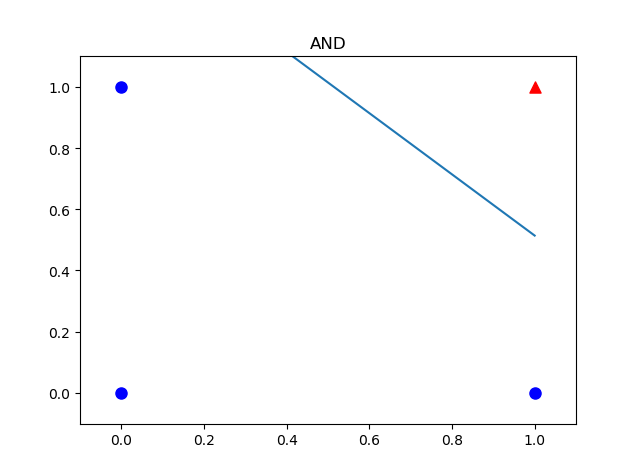
- Output
epoch= 4251
loss= 0.0019995629053717527
w= [[11.76694002 11.76546912]]
b= [[-17.81530488]]
- 逻辑或门分割结果图
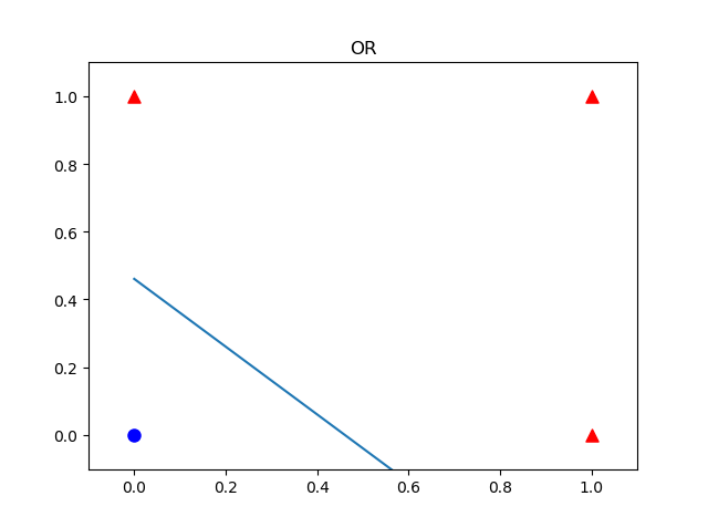
- Output
epoch= 2267
loss= 0.001999175331571145
w= [[11.74573383 11.74749036]]
b= [[-5.41268583]]