人工智能实战2019 第五次作业 续连元

项目	内容
这个作业属于哪个课程	https://edu.cnblogs.com/campus/buaa/BUAA-AI-2019
这个作业的要求在哪里	https://edu.cnblogs.com/campus/buaa/BUAA-AI-2019/homework/2787
我在这个课程的目标是	学习，了解并实践深度学习的实际工程应用
这个作业在哪个具体方面帮助我实现目标	学会用sigmoid激活函数来实现二分类
作业正文	如下
参考文献

正文

一、样本与特征：

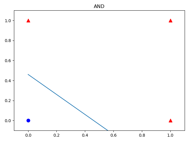
1.逻辑与门
x1=0,x2=0,y=0
x1=0,x2=1,y=0
x1=1,x2=0,y=0
x1=1,x2=1,y=1

2.逻辑或门
x1=0,x2=0,y=0
x1=0,x2=1,y=1
x1=1,x2=0,y=1
x1=1,x2=1,y=1

二、python代码

import numpy as np
import matplotlib.pyplot as plt

def Sigmoid(x):
    s = 1 / (1 + np.exp(-x))
    return s

def ForwardCalculationBatch(W, B, batch_X):
    Z = np.dot(W, batch_X) + B
    A = Sigmoid(Z)
    return A

# 反向计算
def BackPropagationBatch(batch_X, batch_Y, A):
    m = batch_X.shape[1]
    dZ = A - batch_Y
    # dZ列相加，即一行内的所有元素相加
    dB = dZ.sum(axis=1, keepdims=True) / m
    dW = np.dot(dZ, batch_X.T) / m
    return dW, dB

# 更新权重参数
def UpdateWeights(W, B, dW, dB, eta):
    W = W - eta * dW
    B = B - eta * dB
    return W, B

# 计算损失函数值
def CheckLoss(W, B, X, Y):
    m = X.shape[1]
    A = ForwardCalculationBatch(W, B, X)

    p4 = np.multiply(1 - Y, np.log(1 - A))
    p5 = np.multiply(Y, np.log(A))

    LOSS = np.sum(-(p4 + p5))  # binary classification
    loss = LOSS / m
    return loss

# 初始化权重值
def InitialWeights(num_input, num_output):
    W = np.zeros((num_output, num_input))
    B = np.zeros((num_output, 1))
    return W, B


def train(X, Y, ForwardCalculationBatch, CheckLoss):
    num_example = X.shape[1]
    num_feature = X.shape[0]
    num_category = Y.shape[0]
    eta = 0.5
    max_epoch = 10000
    W, B = InitialWeights(num_feature, num_category)
    loss = 5
    error = 2e-3

    for epoch in range(max_epoch):
        for i in range(num_example):
            # get x and y value for one sample
            x = X[:, i].reshape(num_feature, 1)
            y = Y[:, i].reshape(1, 1)
            # get z from x,y
            batch_a = ForwardCalculationBatch(W, B, x)
            # calculate gradient of w and b
            dW, dB = BackPropagationBatch(x, y, batch_a)
            # update w,b
            W, B = UpdateWeights(W, B, dW, dB, eta)
            # end if
        # end for
        # calculate loss for this batch
        loss = CheckLoss(W, B, X, Y)
        while epoch % 300 == 0:
            print(epoch, loss, W, B)
            break
        # end if
        if loss < error:
            print("The final values:", epoch, loss, W, B)
            break
    # end for

    return W, B


def ShowResult(W, B, X, Y, title):
    w = -W[0, 0] / W[0, 1]
    b = -B[0, 0] / W[0, 1]
    x = np.array([0, 1])
    y = w * x + b
    plt.plot(x, y)

    for i in range(X.shape[1]):
        if Y[0, i] == 0:
            plt.scatter(X[0, i], X[1, i], marker="o", c='b', s=64)
        else:
            plt.scatter(X[0, i], X[1, i], marker="^", c='r', s=64)
    plt.axis([-0.1, 1.1, -0.1, 1.1])
    plt.title(title)
    plt.show()


def Read_AND_Data():
    X = np.array([0,0,1,1,0,1,0,1]).reshape(2,4)
    Y = np.array([0,0,0,1]).reshape(1,4)
    return X,Y


def Read_OR_Data():
    X = np.array([0,0,1,1,0,1,0,1]).reshape(2,4)
    Y = np.array([0,1,1,1]).reshape(1,4)
    return X,Y


if __name__ == '__main__':

    # read data
    X,Y = Read_AND_Data()
    #X,Y = Read_OR_Data()
    W, B = train(X, Y, ForwardCalculationBatch, CheckLoss)
    print("w=",W)
    print("b=",B)
    ShowResult(W,B,X,Y,"AND")
#   ShowResult(W,B,X,Y,"OR")

• 运行结果
  逻辑与门：
  0 0.6245484575236854 [[0.18011784 0.15364302]] [[-0.28879391]]
  300 0.027339685455466577 [[6.52272529 6.50253583]] [[-9.90697882]]
  600 0.013975165664463551 [[7.87148038 7.86117736]] [[-11.95217533]]
  900 0.009376095204375197 [[8.67221962 8.66531253]] [[-13.16092597]]
  1200 0.007051854836148108 [[9.24327268 9.23808001]] [[-14.02137546]]
  1500 0.005650047903671916 [[9.68732874 9.68316941]] [[-14.68979595]]
  1800 0.004712705600242369 [[10.05067513 10.04720648]] [[-15.23637875]]
  2100 0.0040418937198415635 [[10.35816415 10.35518963]] [[-15.69873146]]
  2400 0.0035381273319316253 [[10.6246911 10.62208758]] [[-16.09936261]]
  2700 0.0031459420488770965 [[10.85989049 10.85757574]] [[-16.45281634]]
  3000 0.00283197534239208 [[11.07035384 11.06827024]] [[-16.76903553]]
  3300 0.0025749566274840623 [[11.26078966 11.25889527]] [[-17.05511842]]
  3600 0.0023606850197692426 [[11.43467858 11.43294191]] [[-17.31630961]]
  3900 0.002179317929049387 [[11.59466624 11.59306305]] [[-17.55659399]]
  4200 0.00202381848105744 [[11.74281065 11.7413219 ]] [[-17.77907031]]

The final values: 4251 0.0019995629053717527 [[11.76694002 11.76546912]] [[-17.81530488]]

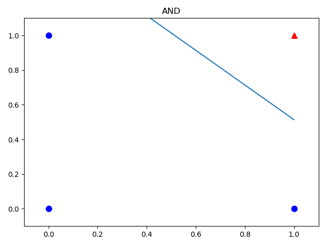
逻辑或门：
0 0.4729860470260927 [[0.40065629 0.43563026]] [[0.43174454]]
300 0.015295923172448746 [[7.65285426 7.66552765]] [[-3.35216603]]
600 0.007618291957258146 [[9.06017234 9.06669204]] [[-4.06406698]]
900 0.005064017080305972 [[9.88144399 9.88582783]] [[-4.47737733]]
1200 0.0037905587598134403 [[10.46298983 10.46629092]] [[-4.76947084]]
1500 0.003028210901112515 [[10.91342626 10.9160732 ]] [[-4.99547549]]
1800 0.0025208676966291367 [[11.28106679 11.28327582]] [[-5.17981738]]
2100 0.00215898093382287 [[11.59164557 11.59354095]] [[-5.33547799]]

The final values: 2267 0.001999175331571145 [[11.74573383 11.74749036]] [[-5.41268583]]