机器学习实战3.3之差分法和ARIMA模型

版权声明：此文章有作者原创，涉及相关版本问题可以联系作者，[email protected] https://blog.csdn.net/weixin_42600072/article/details/88898546

import numpy as np
import pandas as pd
import matplotlib.pyplot as plt
import seaborn as sns

import statsmodels.api as sm
import statsmodels.formula.api as smf
import statsmodels.tsa.api as smt

一些可视化参数设置

pd.set_option('display.float_format', lambda x: '%.5f' % x) # pandas
np.set_printoptions(precision=5, suppress=True) # numpy

pd.set_option('display.max_columns', 100)
pd.set_option('display.max_rows', 100)

# seaborn plotting style
sns.set(style='ticks', context='poster')

导入数据

Sentiment = './data/sentiment.csv'
Sentiment = pd.read_csv(Sentiment, index_col=0, parse_dates=[0])
print(Sentiment.head())

             UMCSENT
DATE                
2000-01-01 112.00000
2000-02-01 111.30000
2000-03-01 107.10000
2000-04-01 109.20000
2000-05-01 110.70000

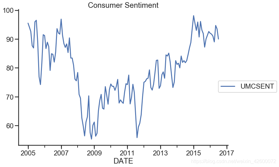
差分法（一般一阶查分就可以了）

#选择数据中一些序列
sentiment_short = Sentiment.loc['2005':'2016']

sentiment_short.plot(figsize=(12,8))
plt.legend(bbox_to_anchor=(1.25, 0.5))
plt.title('Consumer Sentiment')
sns.despine()

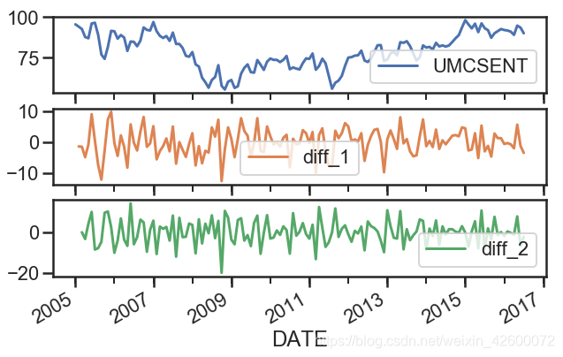
#数字1表示一阶差分，两次一阶差分即可得到两阶差分
sentiment_short['diff_1'] = sentiment_short['UMCSENT'].diff(1)
sentiment_short['diff_2'] = sentiment_short['diff_1'].diff(1)
sentiment_short.plot(subplots=True, figsize=(10,6))

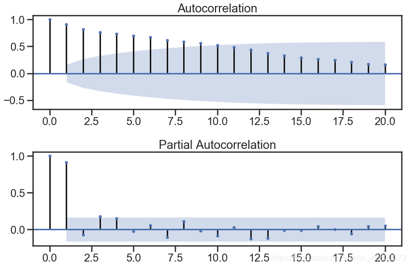
ARIMA模型

• 确定差分阶数d
• ACF函数和PACF函数确定p和q值

del sentiment_short['diff_2']
del sentiment_short['diff_1']
sentiment_short.head()
print (type(sentiment_short))

<class 'pandas.core.frame.DataFrame'>

fig = plt.figure(figsize=(12,8))

ax1 = fig.add_subplot(2,1,1)
fig = sm.graphics.tsa.plot_acf(sentiment_short, lags=20, ax=ax1)
ax1.xaxis.set_ticks_position('bottom')
fig.tight_layout();

ax2 = fig.add_subplot(2,1,2)
fig = sm.graphics.tsa.plot_pacf(sentiment_short, lags=20, ax=ax2)
ax2.xaxis.set_ticks_position('bottom')
fig.tight_layout();

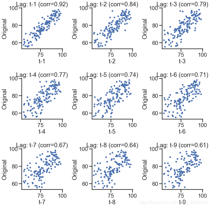
# 散点图也可以表示

lags = 9

ncols = 3
nrows = int(np.ceil(lags / ncols))

fig, axes = plt.subplots(
    ncols=ncols, nrows=nrows, figsize=(4 * ncols, 4 * nrows))

for ax, lag in zip(axes.flat, np.arange(1, lags + 1, 1)):
    lag_str = 't-{}'.format(lag)
    X = (pd.concat(
        [sentiment_short, sentiment_short.shift(-lag)],
        axis=1,
        keys=['y'] + [lag_str]).dropna())

    X.plot(
        ax=ax, kind='scatter', y='y', x=lag_str)
    corr = X.corr().as_matrix()[0][1]
    ax.set_ylabel('Original')
    ax.set_title('Lag: {} (corr={:.2f})'.format(lag_str, corr))
    ax.set_aspect('equal')
    sns.despine()

fig.tight_layout()

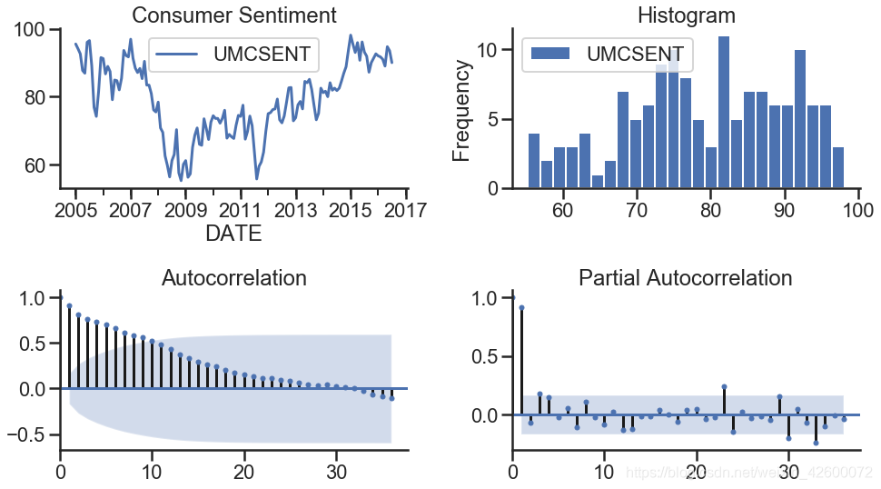
模板画图，直接套用即可

# 更直观一些

def tsplot(y, lags=None, title='', figsize=(14, 8)):

    fig = plt.figure(figsize=figsize)
    layout = (2, 2)
    ts_ax = plt.subplot2grid(layout, (0, 0))
    hist_ax = plt.subplot2grid(layout, (0, 1))
    acf_ax = plt.subplot2grid(layout, (1, 0))
    pacf_ax = plt.subplot2grid(layout, (1, 1))

    y.plot(ax=ts_ax)
    ts_ax.set_title(title)
    y.plot(ax=hist_ax, kind='hist', bins=25)
    hist_ax.set_title('Histogram')
    smt.graphics.plot_acf(y, lags=lags, ax=acf_ax)
    smt.graphics.plot_pacf(y, lags=lags, ax=pacf_ax)
    [ax.set_xlim(0) for ax in [acf_ax, pacf_ax]]
    sns.despine()
    plt.tight_layout()
    return ts_ax, acf_ax, pacf_ax

tsplot(sentiment_short, title='Consumer Sentiment', lags=36)

(<matplotlib.axes._subplots.AxesSubplot at 0x154936a0>,
 <matplotlib.axes._subplots.AxesSubplot at 0x154c47b8>,
 <matplotlib.axes._subplots.AxesSubplot at 0x154e6160>)