[blog] The Illustrated Transformer 2

part1：https://blog.csdn.net/zongza/article/details/88852461

原文：https://jalammar.github.io/illustrated-transformer/

The Beast With Many Heads

The paper further refined the self-attention layer by adding a mechanism called “multi-headed” attention. This improves the performance of the attention layer in two ways:

通过增加一种叫做“多头”注意力（“multi-headed” attention）的机制，论文进一步完善了自注意力层，并在两方面提高了注意力层的性能：

It expands the model’s ability to focus on different positions. Yes, in the example above, z1 contains a little bit of every other encoding, but it could be dominated by the the actual word itself. It would be useful if we’re translating a sentence like “The animal didn’t cross the street because it was too tired”, we would want to know which word “it” refers to.

1.它扩展了模型专注于不同位置的能力。在上面的例子中，虽然每个编码都在z1中有或多或少的体现，但是它可能被实际的单词本身所支配。如果我们翻译一个句子，比如“The animal didn’t cross the street because it was too tired”，我们会想知道“it”指的是哪个词，这时模型的“多头”注意机制会起到作用。

It gives the attention layer multiple “representation subspaces”. As we’ll see next, with multi-headed attention we have not only one, but multiple sets of Query/Key/Value weight matrices (the Transformer uses eight attention heads, so we end up with eight sets for each encoder/decoder). Each of these sets is randomly initialized. Then, after training, each set is used to project the input embeddings (or vectors from lower encoders/decoders) into a different representation subspace.

2.它使得注意力层能拥有多个“表示子空间”（representation subspaces）。（注：表示子空间其实就是上面说的对不同位置的专注能力）接下来我们将看到，对于“多头”注意机制，我们有多个查询/键/值权重矩阵集(Transformer使用八个注意力头，因此我们对于每个编码器/解码器有八个矩阵集合)。这些集合中的每一个都是随机初始化的，在训练之后，每个集合都被用来将输入词嵌入(或来自较低编码器/解码器的向量)投影到不同的表示子空间中。

With multi-headed attention, we maintain separate Q/K/V weight matrices for each head resulting in different Q/K/V matrices. As we did before, we multiply X by the WQ/WK/WV matrices to produce Q/K/V matrices.

在“多头”注意机制下，我们为每个头保持独立的查询/键/值权重矩阵，从而产生不同的查询/键/值矩阵。和之前一样，我们拿X乘以WQ/WK/WV矩阵来产生查询/键/值矩阵。

If we do the same self-attention calculation we outlined above, just eight different times with different weight matrices, we end up with eight different Z matrices

如果我们做与上述相同的自注意力计算，只需八次不同的权重矩阵运算，我们就会得到八个不同的Z矩阵。

This leaves us with a bit of a challenge. The feed-forward layer is not expecting eight matrices – it’s expecting a single matrix (a vector for each word). So we need a way to condense these eight down into a single matrix.

这给我们带来了一点挑战。前馈层不需要8个矩阵，它只需要一个矩阵(由每一个单词的表示向量组成)。所以我们需要一种方法把这八个矩阵压缩成一个矩阵。那该怎么做？其实可以直接把这些矩阵拼接在一起，然后用一个附加的权重矩阵WO与它们相乘。

How do we do that? We concat the matrices then multiple them by an additional weights matrix WO.

That’s pretty much all there is to multi-headed self-attention. It’s quite a handful of matrices, I realize. Let me try to put them all in one visual so we can look at them in one place

这几乎就是多头自注意力的全部。这确实有好多矩阵，我们试着把它们集中在一个图片中，这样可以一眼看清。

Now that we have touched upon attention heads, let’s revisit our example from before to see where the different attention heads are focusing as we encode the word “it” in our example sentence:

既然我们已经摸到了注意力机制的这么多“头”，那么让我们重温之前的例子，看看我们在例句中编码“it”一词时，不同的注意力“头”集中在哪里：

As we encode the word "it", one attention head is focusing most on "the animal", while another is focusing on "tired" -- in a sense, the model's representation of the word "it" bakes in some of the representation of both "animal" and "tired".

当我们编码“it”一词时，一个注意力头集中在“animal”上，而另一个则集中在“tired”上，从某种意义上说，模型对“it”一词的表达在某种程度上是“animal”和“tired”的代表。

If we add all the attention heads to the picture, however, things can be harder to interpret:

然而，如果我们把所有的attention都加到图示里，事情就更难解释了：

Representing The Order of The Sequence Using Positional Encoding

One thing that’s missing from the model as we have described it so far is a way to account for the order of the words in the input sequence.

到目前为止，我们对模型的描述缺少了一种理解输入单词顺序的方法。

To address this, the transformer adds a vector to each input embedding. These vectors follow a specific pattern that the model learns, which helps it determine the position of each word, or the distance between different words in the sequence. The intuition here is that adding these values to the embeddings provides meaningful distances between the embedding vectors once they’re projected into Q/K/V vectors and during dot-product attention.

为了解决这个问题，Transformer为每个输入的词嵌入添加了一个向量。这些向量遵循模型学习到的特定模式，这有助于确定每个单词的位置，或序列中不同单词之间的距离。这里的直觉是，将位置向量添加到词嵌入中使得它们在接下来的运算中，能够更好地表达的词与词之间的距离。

To give the model a sense of the order of the words, we add positional encoding vectors -- the values of which follow a specific pattern.

为了让模型理解单词的顺序，我们添加了位置编码向量，这些向量的值遵循特定的模式。

If we assumed the embedding has a dimensionality of 4, the actual positional encodings would look like this:

如果我们假设词嵌入的维数为4，则实际的位置编码如下：

A real example of positional encoding with a toy embedding size of 4

What might this pattern look like?

这个模式会是什么样子？

In the following figure, each row corresponds the a positional encoding of a vector. So the first row would be the vector we’d add to the embedding of the first word in an input sequence. Each row contains 512 values – each with a value between 1 and -1. We’ve color-coded them so the pattern is visible.

在下图中，每一行对应一个词向量的位置编码，所以第一行对应着输入序列的第一个词。每行包含512个值，每个值介于1和-1之间。我们已经对它们进行了颜色编码，所以图案是可见的。

A real example of positional encoding for 20 words (rows) with an embedding size of 512 (columns). You can see that it appears split in half down the center. That's because the values of the left half are generated by one function (which uses sine), and the right half is generated by another function (which uses cosine). They're then concatenated to form each of the positional encoding vectors.

20字(行)的位置编码实例，词嵌入大小为512(列)。你可以看到它从中间分裂成两半。这是因为左半部分的值由一个函数(使用正弦)生成，而右半部分由另一个函数(使用余弦)生成。然后将它们拼在一起而得到每一个位置编码向量。

The formula for positional encoding is described in the paper (section 3.5). You can see the code for generating positional encodings in get_timing_signal_1d(). This is not the only possible method for positional encoding. It, however, gives the advantage of being able to scale to unseen lengths of sequences (e.g. if our trained model is asked to translate a sentence longer than any of those in our training set).

原始论文里描述了位置编码的公式(第3.5节)。你可以在 get_timing_signal_1d()中看到生成位置编码的代码。这不是唯一可能的位置编码方法。然而，它的优点是能够扩展到未知的序列长度(例如，当我们训练出的模型需要翻译远比训练集里的句子更长的句子时)。

The Residuals

One detail in the architecture of the encoder that we need to mention before moving on, is that each sub-layer (self-attention, ffnn) in each encoder has a residual connection around it, and is followed by a layer-normalization step.

在继续进行下去之前，我们需要提到一个编码器架构中的细节：在每个编码器中的每个子层（自注意力、前馈网络）的周围都有一个残差连接，并且都跟随着一个“层-归一化”步骤。

If we’re to visualize the vectors and the layer-norm operation associated with self attention, it would look like this:

如果我们去可视化这些向量以及这个和自注意力相关联的层-归一化操作，那么看起来就像下面这张图描述一样：

This goes for the sub-layers of the decoder as well. If we’re to think of a Transformer of 2 stacked encoders and decoders, it would look something like this:

解码器的子层也是这样样的。如果我们想象一个2 层编码-解码结构的transformer，它看起来会像下面这张图一样：

The Decoder Side

Now that we’ve covered most of the concepts on the encoder side, we basically know how the components of decoders work as well. But let’s take a look at how they work together.

既然我们已经谈到了大部分编码器的概念，那么我们基本上也就知道解码器是如何工作的了。现在让我们来看看解码器和编码器如何一起工作。

The encoder start by processing the input sequence. The output of the top encoder is then transformed into a set of attention vectors K and V. These are to be used by each decoder in its “encoder-decoder attention” layer which helps the decoder focus on appropriate places in the input sequence:

编码器通过处理输入序列开启工作。顶端编码器的输出之后会变转化为一个包含向量K（键向量）和V（值向量）的注意力向量集。这些向量将被每个解码器用于自身的“编码-解码注意力层”，而这些层可以帮助解码器从输入序列中取出query想要查询的位置处的信息：

After finishing the encoding phase, we begin the decoding phase. Each step in the decoding phase outputs an element from the output sequence (the English translation sentence in this case).

在完成编码阶段后，则开始解码阶段。解码阶段的每个步骤都会得到输出序列中的一个元素（在这个例子里，是英语翻译的句子）（注：decoder的每一步输出都会作为下一步的输入，decoder原始输入应该是一个固定的表示开始的单词）

The following steps repeat the process until a special symbol is reached indicating the transformer decoder has completed its output. The output of each step is fed to the bottom decoder in the next time step, and the decoders bubble up their decoding results just like the encoders did. And just like we did with the encoder inputs, we embed and add positional encoding to those decoder inputs to indicate the position of each word.

接下来的步骤重复了这个过程，直到到达一个特殊的终止符号，它表示transformer的解码器已经完成了它的输出。每个步骤的输出在下一个时间步被提供给底端解码器，并且就像编码器之前做的那样，这些解码器会输出它们的解码结果。另外，就像我们对编码器的输入所做的那样，我们会嵌入并添加位置编码给那些解码器，来表示每个单词的位置。

The self attention layers in the decoder operate in a slightly different way than the one in the encoder:

In the decoder, the self-attention layer is only allowed to attend to earlier positions in the output sequence. This is done by masking future positions (setting them to -inf) before the softmax step in the self-attention calculation.

而那些解码器中的自注意力层表现的模式与编码器不同：在解码器中，自注意力层只被允许处理输出序列中当前单词之前的那些位置。（注：在softmax步骤前，通过把它们设为-inf把后面的位置给隐去）

The “Encoder-Decoder Attention” layer works just like multiheaded self-attention, except it creates its Queries matrix from the layer below it, and takes the Keys and Values matrix from the output of the encoder stack.

这个“编码-解码注意力层”工作方式基本就像多头自注意力层一样，只不过它是通过在decoder的self层来创造查询矩阵，从encoder的输出中取得键/值矩阵。

The Final Linear and Softmax Layer

The decoder stack outputs a vector of floats. How do we turn that into a word? That’s the job of the final Linear layer which is followed by a Softmax Layer.

解码组件最后会输出一个实数向量。我们如何把浮点数变成一个单词？这便是线性变换层要做的工作，它之后就是Softmax层。

The Linear layer is a simple fully connected neural network that projects the vector produced by the stack of decoders, into a much, much larger vector called a logits vector.

线性变换层是一个简单的全连接神经网络，它可以把解码组件产生的向量投射到一个比它大得多的、被称作对数几率（logits）的向量里。

Let’s assume that our model knows 10,000 unique English words (our model’s “output vocabulary”) that it’s learned from its training dataset. This would make the logits vector 10,000 cells wide – each cell corresponding to the score of a unique word. That is how we interpret the output of the model followed by the Linear layer.

不妨假设我们的模型从训练集中学习一万个不同的英语单词（我们模型的“输出词表”）。因此对数几率向量为一万个单元格长度的向量——每个单元格对应某一个单词的分数。

The softmax layer then turns those scores into probabilities (all positive, all add up to 1.0). The cell with the highest probability is chosen, and the word associated with it is produced as the output for this time step.

接下来的Softmax 层便会把那些分数变成概率（都为正数、上限1.0）。概率最高的单元格被选中，并且它对应的单词被作为这个时间步的输出。

This figure starts from the bottom with the vector produced as the output of the decoder stack. It is then turned into an output word.

这张图片从底部以解码器组件产生的输出向量开始。之后它会转化出一个输出单词。

Recap Of Training

Now that we’ve covered the entire forward-pass process through a trained Transformer, it would be useful to glance at the intuition of training the model.

既然我们已经过了一遍完整的transformer的前向传播过程，那我们就可以直观感受一下它的训练过程。

During training, an untrained model would go through the exact same forward pass. But since we are training it on a labeled training dataset, we can compare its output with the actual correct output.

在训练过程中，一个未经训练的模型会通过一个完全一样的前向传播。但因为我们用有标记的训练集来训练它，所以我们可以用它的输出去与真实的输出做比较。

To visualize this, let’s assume our output vocabulary only contains six words(“a”, “am”, “i”, “thanks”, “student”, and “<eos>” (short for ‘end of sentence’)).

为了把这个流程可视化，不妨假设我们的输出词汇仅仅包含六个单词：“a”, “am”, “i”, “thanks”, “student”以及 “<eos>”（end of sentence的缩写形式）。

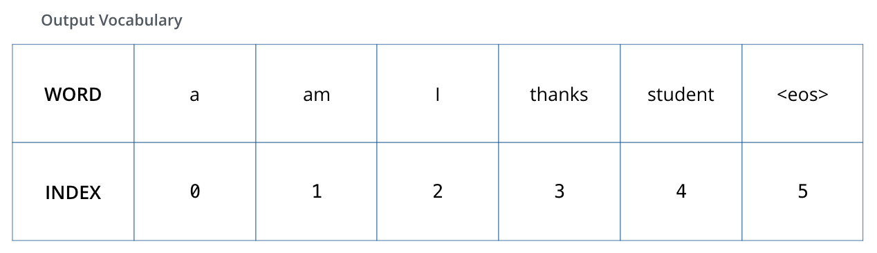
The output vocabulary of our model is created in the preprocessing phase before we even begin training.

我们模型的输出词表在我们训练之前的预处理流程中就被设定好。

Once we define our output vocabulary, we can use a vector of the same width to indicate each word in our vocabulary. This also known as one-hot encoding. So for example, we can indicate the word “am” using the following vector:

一旦我们定义了我们的输出词表，我们可以使用一个相同宽度的向量来表示我们词汇表中的每一个单词。这也被认为是一个one-hot 编码。所以，我们可以用下面这个向量来表示单词“am”：

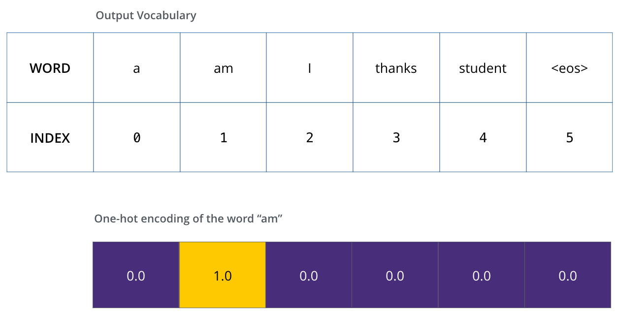
Example: one-hot encoding of our output vocabulary

Following this recap, let’s discuss the model’s loss function – the metric we are optimizing during the training phase to lead up to a trained and hopefully amazingly accurate model.

接下来我们讨论模型的损失函数——这是我们用来在训练过程中优化的标准。通过它可以训练得到一个结果尽量准确的模型。

The Loss Function

Say we are training our model. Say it’s our first step in the training phase, and we’re training it on a simple example – translating “merci” into “thanks”.

比如说我们正在训练模型，现在是第一步，一个简单的例子——把“merci”翻译为“thanks”。

What this means, is that we want the output to be a probability distribution indicating the word “thanks”. But since this model is not yet trained, that’s unlikely to happen just yet.

这意味着我们想要一个表示单词“thanks”概率分布的输出。但是因为这个模型还没被训练好，所以不太可能现在就出现这个结果。

Since the model's parameters (weights) are all initialized randomly, the (untrained) model produces a probability distribution with arbitrary values for each cell/word. We can compare it with the actual output, then tweak all the model's weights using backpropagation to make the output closer to the desired output.

因为模型的参数（权重）都被随机的生成，（未经训练的）模型产生的概率分布在每个单元格/单词里都赋予了随机的数值。我们可以用真实的输出来比较它，然后用反向传播算法来略微调整所有模型的权重，生成更接近结果的输出。

How do you compare two probability distributions? We simply subtract one from the other. For more details, look atcross-entropy and Kullback–Leibler divergence.

你会如何比较两个概率分布呢？我们可以简单地用其中一个减去另一个。更多细节请参考交叉熵和KL散度。

But note that this is an oversimplified example. More realistically, we’ll use a sentence longer than one word. For example – input: “je suis étudiant” and expected output: “i am a student”. What this really means, is that we want our model to successively output probability distributions where:

但注意到这是一个过于简化的例子。更现实的情况是处理一个句子。例如，输入“je suis étudiant”并期望输出是“i am a student”。那我们就希望我们的模型能够成功地在这些情况下输出概率分布：

Each probability distribution is represented by a vector of width vocab_size (6 in our toy example, but more realistically a number like 3,000 or 10,000)
The first probability distribution has the highest probability at the cell associated with the word “i”
The second probability distribution has the highest probability at the cell associated with the word “am”
And so on, until the fifth output distribution indicates ‘<end of sentence>’ symbol, which also has a cell associated with it from the 10,000 element vocabulary.

每个概率分布被一个以词表大小（我们的例子里是6，但现实情况通常是3000或10000）为宽度的向量所代表。

第一个概率分布在与“i”关联的单元格有最高的概率

第二个概率分布在与“am”关联的单元格有最高的概率

以此类推，第五个输出的分布表示“<end of sentence>”关联的单元格有最高的概率

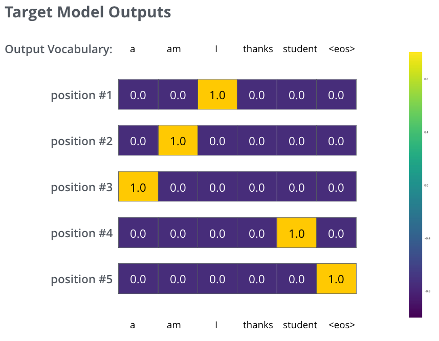
The targeted probability distributions we'll train our model against in the training example for one sample sentence.

依据例子训练模型得到的目标概率分布。

After training the model for enough time on a large enough dataset, we would hope the produced probability distributions would look like this:

在一个足够大的数据集上充分训练后，我们希望模型输出的概率分布看起来像这个样子：

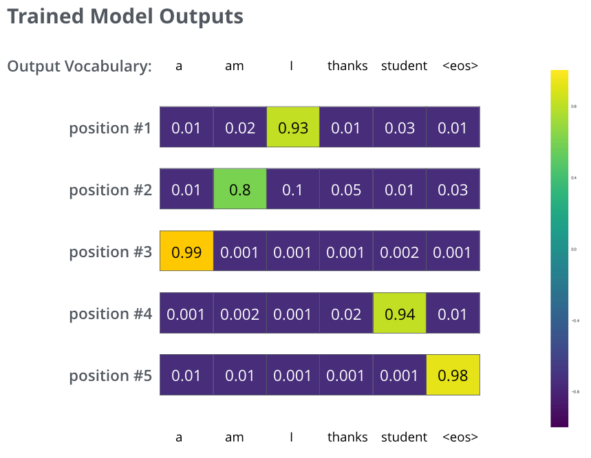
Hopefully upon training, the model would output the right translation we expect. Of course it's no real indication if this phrase was part of the training dataset (see: cross validation). Notice that every position gets a little bit of probability even if it's unlikely to be the output of that time step -- that's a very useful property of softmax which helps the training process.

我们期望训练过后，模型会输出正确的翻译。当然如果这段话完全来自训练集，它并不是一个很好的评估指标（参考：交叉验证，链接https://www.youtube.com/watch?v=TIgfjmp-4BA）。注意到每个位置（词）都得到了一点概率，即使它不太可能成为那个时间步的输出——这是softmax的一个很有用的性质，它可以帮助模型训练。

Now, because the model produces the outputs one at a time, we can assume that the model is selecting the word with the highest probability from that probability distribution and throwing away the rest. That’s one way to do it (called greedy decoding). Another way to do it would be to hold on to, say, the top two words (say, ‘I’ and ‘a’ for example), then in the next step, run the model twice: once assuming the first output position was the word ‘I’, and another time assuming the first output position was the word ‘me’, and whichever version produced less error considering both positions #1 and #2 is kept. We repeat this for positions #2 and #3…etc. This method is called “beam search”, where in our example, beam_size was two (because we compared the results after calculating the beams for positions #1 and #2), and top_beams is also two (since we kept two words). These are both hyperparameters that you can experiment with.

因为这个模型一次只产生一个输出，不妨假设这个模型只选择概率最高的单词，并把剩下的词抛弃。这是其中一种方法（叫贪心解码）。另一个完成这个任务的方法是留住概率最靠高的两个单词（例如I和a），那么在下一步里，跑模型两次：其中一次假设第一个位置输出是单词“I”，而另一次假设第一个位置输出是单词“me”，并且无论哪个版本产生更少的误差，都保留概率最高的两个翻译结果。然后我们为第二和第三个位置重复这一步骤。这个方法被称作集束搜索（beam search）。在我们的例子中，集束宽度是2（因为保留了2个集束的结果，如第一和第二个位置），并且最终也返回两个集束的结果（top_beams也是2）。这些都是可以提前设定的参数。

Go Forth And Transform

I hope you’ve found this a useful place to start to break the ice with the major concepts of the Transformer. If you want to go deeper, I’d suggest these next steps:

我希望通过上文已经让你们了解到Transformer的主要概念了。如果你想在这个领域深入，我建议可以走以下几步：阅读Attention Is All You Need，Transformer博客和Tensor2Tensor announcement，以及看看Łukasz Kaiser的介绍，了解模型和细节。

Read the Attention Is All You Need paper, the Transformer blog post (Transformer: A Novel Neural Network Architecture for Language Understanding), and the Tensor2Tensor announcement.
Watch Łukasz Kaiser’s talk walking through the model and its details
Play with the Jupyter Notebook provided as part of the Tensor2Tensor repo
Explore the Tensor2Tensor repo.

Follow-up works:

接下来可以研究的工作：