基于前面的随机森林做分类任务
https://blog.csdn.net/qq_40229367/article/details/88526749
我们看一下数据与特征对随机森林的影响
我们读入一个数据量更多,特征也多了的数据集
import pandas as pd
# Read in data as a dataframe
features = pd.read_csv('data/temps_extended.csv')
features.head(5)
print('We have {} days of data with {} variables.'.format(*features.shape))
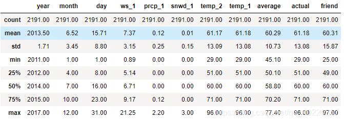
round(features.describe(), 2)
前面我们知道了重要性最大的一个特征temp_1,这是前一天的气温
我们新加入了
- ws_1:前一天的风速
- prcp_1: 前一天的降水
- snwd_1:前一天的积雪深度
此时的数据情况:
We have 2191 days of data with 12 variables.
和前面文章一个类似的操作,合并了一些相关性强的特征(year month day),然后选择某些特征画图看一下数据情况
import datetime

# Get years, months, and days
years = features['year']
months = features['month']
days = features['day']

# List and then convert to datetime object
dates =
[str(int(year)) + '-' + str(int(month)) + '-' + str(int(day)) for year, month, day in zip(years, months, days)]
dates = [datetime.datetime.strptime(date, '%Y-%m-%d') for date in dates]

# Import matplotlib for plotting and use magic command for Jupyter Notebooks
import matplotlib.pyplot as plt

%matplotlib inline

# Set the style
plt.style.use('fivethirtyeight')

# Set up the plotting layout
fig, ((ax1, ax2), (ax3, ax4)) = plt.subplots(nrows=2, ncols=2, figsize = (15,10))
fig.autofmt_xdate(rotation = 45)

# Actual max temperature measurement
ax1.plot(dates, features['actual'])
ax1.set_xlabel(''); ax1.set_ylabel('Temperature (F)'); ax1.set_title('Max Temp')

# Temperature from 1 day ago
ax2.plot(dates, features['temp_1'])
ax2.set_xlabel(''); ax2.set_ylabel('Temperature (F)'); ax2.set_title('Prior Max Temp')

# Temperature from 2 days ago
ax3.plot(dates, features['temp_2'])
ax3.set_xlabel('Date'); ax3.set_ylabel('Temperature (F)'); ax3.set_title('Two Days Prior Max Temp')

# Friend Estimate
ax4.plot(dates, features['friend'])
ax4.set_xlabel('Date'); ax4.set_ylabel('Temperature (F)'); ax4.set_title('Friend Estimate')

plt.tight_layout(pad=2)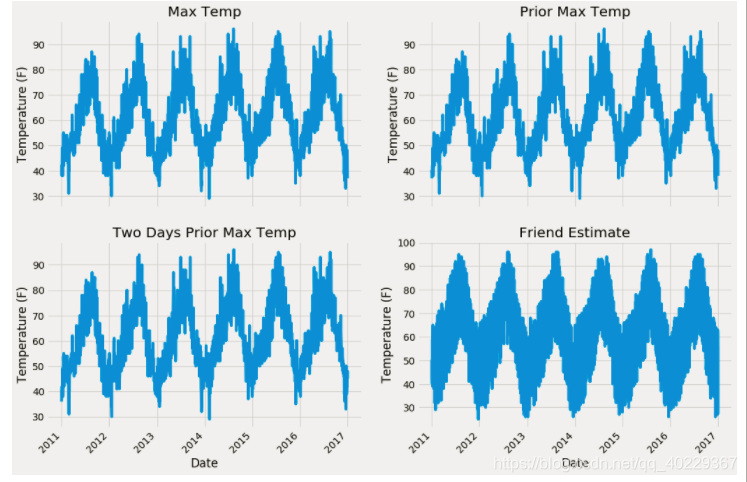
可以看到这里的数据变成了2011-2017年的数据了
再来看下新加入的特征的情况
# Set up the plotting layout
fig, ((ax1, ax2), (ax3, ax4)) = plt.subplots(nrows=2, ncols=2, figsize = (15,10))
fig.autofmt_xdate(rotation = 45)

# Historical Average Max Temp
ax1.plot(dates, features['average'])
ax1.set_xlabel(''); ax1.set_ylabel('Temperature (F)'); ax1.set_title('Historical Avg Max Temp')

# Prior Avg Wind Speed
ax2.plot(dates, features['ws_1'], 'r-')
ax2.set_xlabel(''); ax2.set_ylabel('Wind Speed (mph)'); ax2.set_title('Prior Wind Speed')

# Prior Precipitation
ax3.plot(dates, features['prcp_1'], 'r-')
ax3.set_xlabel('Date'); ax3.set_ylabel('Precipitation (in)'); ax3.set_title('Prior Precipitation')

# Prior Snowdepth
ax4.plot(dates, features['snwd_1'], 'ro')
ax4.set_xlabel('Date'); ax4.set_ylabel('Snow Depth (in)'); ax4.set_title('Prior Snow Depth')

plt.tight_layout(pad=2)
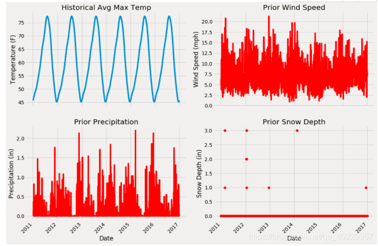
你看出来了什么吗。我。还看不出来什么,就是第一个图出现最大值、数据爬升下降趋势每年都是差不多的。
之后我们还可以用pairplot,将特征两两组合对比,看之间的关系
# Create columns of seasons for pair plotting colors
seasons = []

for month in features['month']:
    if month in [1, 2, 12]:
        seasons.append('winter')
    elif month in [3, 4, 5]:
        seasons.append('spring')
    elif month in [6, 7, 8]:
        seasons.append('summer')
    elif month in [9, 10, 11]:
        seasons.append('fall')

# Will only use six variables for plotting pairs
reduced_features = features[['temp_1', 'prcp_1', 'average', 'actual']]
reduced_features['season'] = seasons

# Use seaborn for pair plots
import seaborn as sns
sns.set(style="ticks", color_codes=True);

# Create a custom color palete
palette = sns.xkcd_palette(['dark blue', 'dark green', 'gold', 'orange'])

# Make the pair plot with a some aesthetic changes
sns.pairplot(reduced_features, hue = 'season', diag_kind = 'kde', palette= palette, plot_kws=dict(alpha = 0.7),
diag_kws=dict(shade=True)); 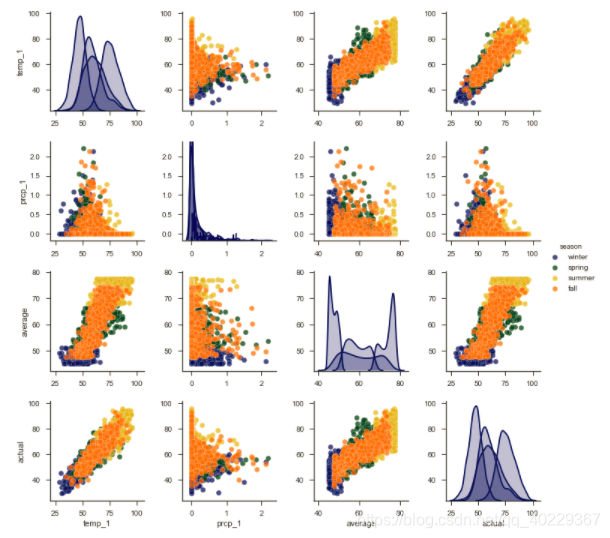
这是分四季来看数据情况,temp_1和average都跟真实情况有着比较强的关系
(中间的是特征自己,只能看四季变化情况)
之后,我们同样进行数据预处理和数据切分
# One Hot Encoding
features = pd.get_dummies(features)

# Extract features and labels
labels = features['actual']
features = features.drop('actual', axis = 1)

# List of features for later use
feature_list = list(features.columns)

# Convert to numpy arrays
import numpy as np

features = np.array(features)
labels = np.array(labels)

# Training and Testing Sets
from sklearn.model_selection import train_test_split

train_features, test_features, train_labels, test_labels =
 train_test_split(features, labels,
test_size = 0.25, random_state = 42)

print('Training Features Shape:', train_features.shape)
print('Training Labels Shape:', train_labels.shape)
print('Testing Features Shape:', test_features.shape)
print('Testing Labels Shape:', test_labels.shape)
Training Features Shape: (1643, 17) Training Labels Shape: (1643,) Testing Features Shape: (548, 17) Testing Labels Shape: (548,)
而我们前面得到的结果是
Average model error: 3.83 degrees.
Accuracy: 93.99 %.
此时我们仅增大数据量(先忽略新特征)来比较一下
from sklearn.ensemble import RandomForestRegressor
# Find the original feature indices
original_feature_indices = [feature_list.index(feature) for feature in
                                      feature_list if feature not in
                                      ['ws_1', 'prcp_1', 'snwd_1']]

# Create a test set of the original features
original_train_features = train_features[:,original_feature_indices]

original_test_features = test_features[:, original_feature_indices]

rf = RandomForestRegressor(n_estimators= 100, random_state=42)

rf.fit(original_train_features, train_labels);

# Make predictions on test data using the model trained on original data
baseline_predictions = rf.predict(original_test_features)

# Performance metrics
baseline_errors = abs(baseline_predictions - test_labels)

print('Metrics for Random Forest Trained on Original Data')
print('Average absolute error:', round(np.mean(baseline_errors), 2), 'degrees.')

# Calculate mean absolute percentage error (MAPE)
baseline_mape = 100 * np.mean((baseline_errors / test_labels))

# Calculate and display accuracy
baseline_accuracy = 100 - baseline_mape
print('Accuracy:', round(baseline_accuracy, 2), '%.')
Metrics for Random Forest Trained on Original Data Average absolute error: 3.75 degrees. Accuracy: 93.7 %.
效果好了一丢丢
那我们再加入新特征来看
from sklearn.ensemble import RandomForestRegressor

rf_exp = RandomForestRegressor(n_estimators= 100, random_state=42)
rf_exp.fit(train_features, train_labels)


# Make predictions on test data
predictions = rf_exp.predict(test_features)

# Performance metrics
errors = abs(predictions - test_labels)

print('Metrics for Random Forest Trained on Expanded Data')
print('Average absolute error:', round(np.mean(errors), 4), 'degrees.')

# Calculate mean absolute percentage error (MAPE)
mape = np.mean(100 * (errors / test_labels))

# Compare to baseline
improvement_baseline = 100 * abs(mape - baseline_mape) / baseline_mape
print('Improvement over baseline:', round(improvement_baseline, 2), '%.')

# Calculate and display accuracy
accuracy = 100 - mape
print('Accuracy:', round(accuracy, 2), '%.')
Metrics for Random Forest Trained on Expanded Data Average absolute error: 3.7162 degrees. Improvement over baseline: 0.48 %. Accuracy: 93.73 %.
又提升了一点
那么其实我们可以知道,数据量多,相关特征越多,就预测越准
但是数据量和特征越多,那么运行的时间越久越长吧
我们就像需要考虑性价比的问题(在不同问题中偏重是不一样的)
那么假如我们现在需要进行特征降维,选择前95%的特征进行训练
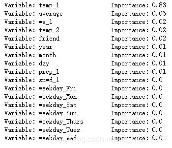
同样先来看下特征重要性
# Get numerical feature importances
importances = list(rf_exp.feature_importances_)

# List of tuples with variable and importance
feature_importances = [(feature, round(importance, 2)) for feature, importance in zip(feature_list, importances)]

# Sort the feature importances by most important first
feature_importances = sorted(feature_importances, key = lambda x: x[1], reverse = True)

# Print out the feature and importances
[print('Variable: {:20} Importance: {}'.format(*pair)) for pair in feature_importances];
# Reset style
plt.style.use('fivethirtyeight')

# list of x locations for plotting
x_values = list(range(len(importances)))

# Make a bar chart
plt.bar(x_values, importances, orientation = 'vertical', color = 'r', edgecolor = 'k', linewidth = 1.2)

# Tick labels for x axis
plt.xticks(x_values, feature_list, rotation='vertical')

# Axis labels and title
plt.ylabel('Importance'); plt.xlabel('Variable'); plt.title('Variable Importances');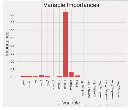
之后选择给特征进行cumsum和排序,选择前面能实现95%以上的特征
# List of features sorted from most to least important
sorted_importances = [importance[1] for importance in feature_importances]
sorted_features = [importance[0] for importance in feature_importances]

# Cumulative importances
cumulative_importances = np.cumsum(sorted_importances)

# Make a line graph
plt.plot(x_values, cumulative_importances, 'g-')

# Draw line at 95% of importance retained
plt.hlines(y = 0.95, xmin=0, xmax=len(sorted_importances), color = 'r', linestyles = 'dashed')

# Format x ticks and labels
plt.xticks(x_values, sorted_features, rotation = 'vertical')

# Axis labels and title
plt.xlabel('Variable'); plt.ylabel('Cumulative Importance'); plt.title('Cumulative Importances');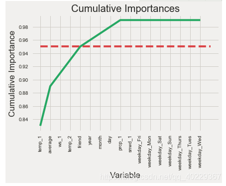
# Find number of features for cumulative importance of 95%
# Add 1 because Python is zero-indexed
print('Number of features for 95% importance:',
np.where(cumulative_importances > 0.95)[0][0] + 1)
Number of features for 95% importance: 6
那么我们就选择前六个特征来作为我们要研究的特征
因为是选择部分特征作为研究,那么我们要重新设定好数据集,之后再分为训练集和测试集,也需要重新训练随机森林
# Extract the names of the most important features
important_feature_names = [feature[0] for feature in feature_importances[0:6]]
# Find the columns of the most important features
important_indices = [feature_list.index(feature) for feature in important_feature_names]

# Create training and testing sets with only the important features
important_train_features = train_features[:, important_indices]
important_test_features = test_features[:, important_indices]

# Sanity check on operations
print('Important train features shape:', important_train_features.shape)
print('Important test features shape:', important_test_features.shape)
Important train features shape: (1643, 6) Important test features shape: (548, 6)
选择特征后重新切分的训练集和测试集
# Train the expanded model on only the important features
rf_exp.fit(important_train_features, train_labels);


# Make predictions on test data
predictions = rf_exp.predict(important_test_features)

# Performance metrics
errors = abs(predictions - test_labels)

print('Average absolute error:', round(np.mean(errors), 4), 'degrees.')

# Calculate mean absolute percentage error (MAPE)
mape = 100 * (errors / test_labels)

# Calculate and display accuracy
accuracy = 100 - np.mean(mape)
print('Accuracy:', round(accuracy, 2), '%.')
Average absolute error: 3.8288 degrees. Accuracy: 93.56 %.
可以看到效果,是比之前差那么一点的,这是因为选择特征少了,数据量也就少了
但我们来比较下时间
# Use time library for run time evaluation
import time
# All features training and testing time
all_features_time = []
# Do 10 iterations and take average for all features
for _ in range(10):
start_time = time.time()
rf_exp.fit(train_features, train_labels)
all_features_predictions = rf_exp.predict(test_features)
end_time = time.time()
all_features_time.append(end_time - start_time)
all_features_time = np.mean(all_features_time)
print('All features total training and testing time:', round(all_features_time, 2), 'seconds.')
# Time training and testing for reduced feature set
reduced_features_time = []
# Do 10 iterations and take average
for _ in range(10):
start_time = time.time()
rf_exp.fit(important_train_features, train_labels)
reduced_features_predictions = rf_exp.predict(important_test_features)
end_time = time.time()
reduced_features_time.append(end_time - start_time)
reduced_features_time = np.mean(reduced_features_time)
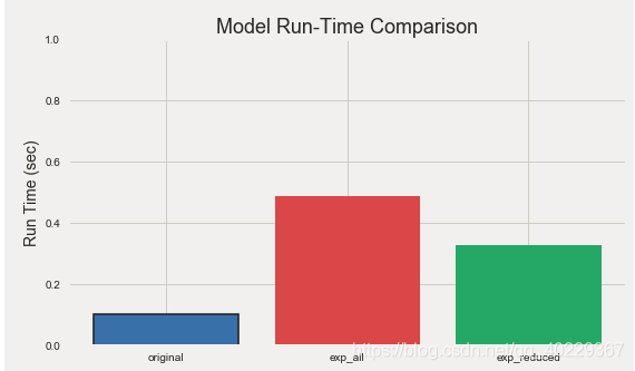
print('Reduced features total training and testing time:', round(reduced_features_time, 2), 'seconds.')All features total training and testing time: 0.49 seconds.
Reduced features total training and testing time: 0.33 seconds.
时间是由平均十次训练得到结果的时间
那么我们来比较下时间和准确率
all_accuracy =  100 * (1- np.mean(abs(all_features_predictions - test_labels) / test_labels))
reduced_accuracy = 100 * (1- np.mean(abs(reduced_features_predictions - test_labels) / test_labels))

comparison = pd.DataFrame({'features': ['all (17)', 'reduced (5)'],
                           'run_time': [round(all_features_time, 2), round(reduced_features_time, 2)],
                           'accuracy': [round(all_accuracy, 2), round(reduced_accuracy, 2)]})

comparison[['features', 'accuracy', 'run_time']]
relative_accuracy_decrease = 100 * (all_accuracy - reduced_accuracy) / all_accuracy
print('Relative decrease in accuracy:', round(relative_accuracy_decrease, 3), '%.')

relative_runtime_decrease = 100 * (all_features_time - reduced_features_time) / all_features_time
print('Relative decrease in run time:', round(relative_runtime_decrease, 3), '%.')
Relative decrease in accuracy: 0.186 %. Relative decrease in run time: 33.197 %.
这里可以看到,准确率只是下降了0.186%但是时间却减少了33.197%
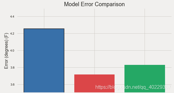
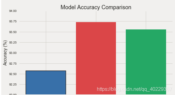
最后我们来比较下,前面文章(相对,数据量少,特征少)和本文章两种模型(数据量多,特征少 和 数据量多,特征多)的效果

0 1 2