以下内容笔记出自‘跟着迪哥学python数据分析与机器学习实战’,外加个人整理添加,仅供个人复习使用。
在上一篇文章进行简单建模的基础上,这里应用的数据量增大,讨论数据量大小与特征使用对随机模型性能大小的影响。
import os
#os.chdir(r'路径')
import pandas as pd
features=pd.read_csv(r'temps_extended.csv')
print(features.shape)
features.head(5)
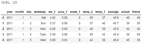
数据集中添加了新变量
ws_1:前一天风速;
prcp_1:前一天降水;
snwd_1:前一天积雪深度;
查看温度图形
import datetime
years=features['year']
months=features['month']
days=features['day']
#格式转换
dates=[str(int(year))+'-'+str(int(month))+ '-'+ str(int(day))
      for year,month,day in zip(years,months,days)]
#作图
import matplotlib.pyplot as plt
%matplotlib inline

#风格设置
#plt.style.use('fivethirtyeight')
fig,((ax1,ax2),(ax3,ax4))=plt.subplots(nrows=2,ncols=2,
                                      figsize=(15,10))

fig.autofmt_xdate(rotation=45)
ax1.plot(dates,features['average'])
ax2.plot(dates,features['ws_1'],'r-')
ax3.plot(dates,features['prcp_1'],'r-')
ax4.plot(dates,features['snwd_1'],'ro')
plt.tight_layout(pad=2)

查看不同季节的温度关系
(这里可以学习下如何新建变量以及作图)
#创建一个新变量season
seasons=[]

for month in features['month']:
    if month in [1,2,12]:
        seasons.append('winter')
    elif month in [3,4,5]:
        seasons.append('spring')
    elif month in [6,7,8]:
        seasons.append('summer')
    elif month in [9,10,11]:
        seasons.append('fall')
import warnings
warnings.filterwarnings('ignore')

reduced_features=features[['temp_1','prcp_1','average','actual']]
reduced_features['season']=seasons
print(reduced_features.shape)
reduced_features.head(6)

查看变量间关系,矩阵图:
#查看变量间关系
import seaborn as sns
sns.set(style='ticks',color_codes=True)

palette=sns.xkcd_palette(['dark blue','dark green',
                         'gold','orange'])

#绘制pairplot
sns.pairplot(reduced_features,hue='season',
            diag_kind='kde',
            palette=palette,
            plot_kws=dict(alpha=0.7),
            diag_kws=dict(shade=True))
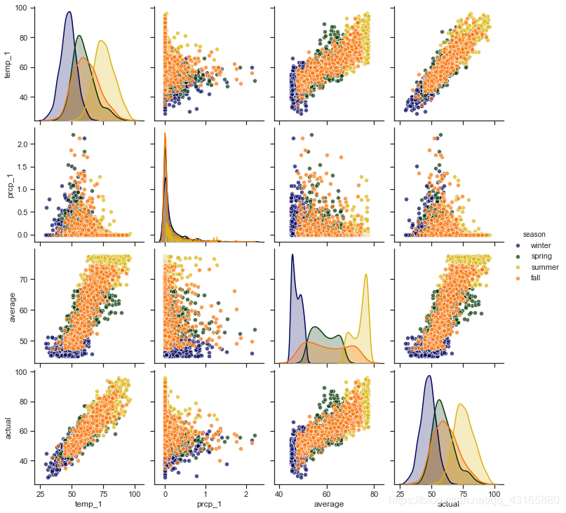
可以看到,x轴和y轴为4项指标,不同颜色表示不同季节,在主对角线上x轴和y轴都是相同特征,表示在不同季节的数值分布情况,其他位置用散点图表示两个特征间的关系。可以看到,左下角temp_1和actual呈现很强相关性。
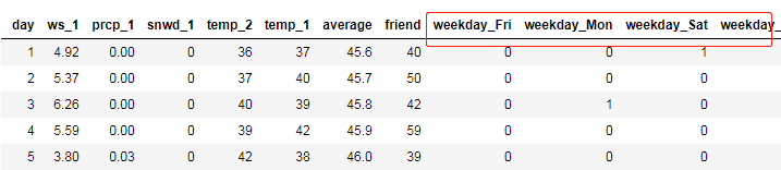
数据预处理

#独热编码
features=pd.get_dummies(features)

#提取特征和标签
labels=features['actual']
features=features.drop('actual',axis=1)
feature_list=list(features.columns)
features.head(2)
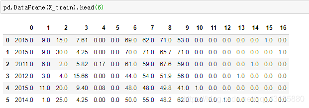
转换格式并进行数据切分:
#转换格式
import numpy as np
features_arr=np.array(features)
labels_arr=np.array(labels)

#数据切分
from sklearn.model_selection import train_test_split
X_train,X_test,y_train,y_test=train_test_split(features_arr,labels_arr,
                                              test_size=0.25,
                                              random_state=0)
print(X_train.shape,X_test.shape)
(1643, 17) (548, 17)
建立模型
这里我们是想看当数据量增多或特征不同时,对模型的影响,因此,这里建立旧模型(使用数据量少、特征少的旧数据集),使用新测试集分别测试旧模型和新模型的效果,来比较模型性能。
旧模型(数据量小,特征少)

#哑变量设置
o_features=pd.get_dummies(o_features)
#数据和标签
o_labels_arr=np.array(o_features['actual'])
o_features_arr=np.array(o_features.drop('actual',axis=1))
o_feature_list=list(o_features.columns)
#切分数据
o_X_train,o_X_test,o_y_train,o_y_test=train_test_split(o_features_arr,
o_labels_arr,
test_size=0.25,
random_state=42)
#建模
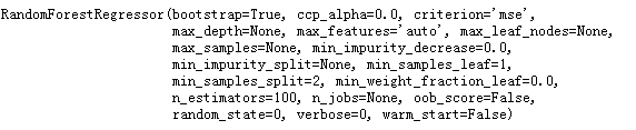
from sklearn.ensemble import RandomForestRegressor
rf=RandomForestRegressor(n_estimators=100,random_state=0)
rf.fit(o_X_train,o_y_train)
使用新测试集来测试,但注意新测试集中的特征多,而旧数据集的特征要少,因此要挑出相应特征:
#老数据集的特征少,这里要选出相应特征
o_features_indices=[feature_list.index(feature) for feature in
                   feature_list if feature not in
                   ['ws_1','prcp_1','snwd_1']]  #返回索引值
predictions=rf.predict(X_test[:,o_features_indices])

#计算误差
errors=abs(predictions-y_test)
print('平均温度误差:',round(np.mean(errors),2),'degrees.')

#MAPE
mape=100*(errors/y_test)  #每个点误差率
#返回accuracy
accuracy=100-np.mean(mape)
print('Accuracy',round(accuracy,2),'%.')
平均温度误差: 4.67 degrees.
Accuracy 92.2 %.
注意模型是回归模型,模型性能使用平均误差来衡量,这里的准确率只是一个叫法(好像不太合适,先这样称呼吧),是减去误差率得出的结果,与分类模型中的准确率计算方式不同。
可以看到,旧模型的平均绝对误差为4.67,准确率为92.2%。
新模型(数据量增大,特征不变)
注意,这里:
o_X_train,o_y_train 老数据集
o_feature_list 变量索引
X_train,y_train 新数据集
feature_list 变量索引
max_X_train=X_train[:,o_features_indices]
#特征选择原特征,但数据量是增多的
max_X_test=X_test[:,o_features_indices]

rf=RandomForestRegressor(n_estimators=100,random_state=0)
rf.fit(max_X_train,y_train)

#预测
max_predictions=rf.predict(max_X_test)
#误差
max_errors=abs(max_predictions-y_test)
print('平均误差:',round(np.mean(max_errors),2),'degree.')

max_mape=100*np.mean((max_errors/y_test))
max_acc=100-max_mape
print('Accuracy:',round(max_acc,2),'%.')
平均误差: 4.2 degree.
Accuracy: 93.12 %.
在这个例子中,数据量增多后,拟合模型的性能提高了,平均误差减低了0.47
新模型(数据量增多,特征增多)
也就是直接使用篇头导入的新数据集建模

#同样测试集
predictions=fina_rf.predict(X_test)
errors=abs(predictions-y_test)
print('平均误差:',round(np.mean(errors),2),'degrees.')

mape=np.mean(100*(errors / y_test))
#看下提升了多少
improve=100*abs(mape-max_mape)/max_mape
print('特征增多后模型效果提升:',round(improve,2),'%.')

#accuracy
accuracy=100-mape
print('准确率:',round(accuracy,2),'%.')
平均误差: 4.05 degrees.
特征增多后模型效果提升: 3.34 %.
准确率: 93.35 %.
可以看到,模型整体效果有了提升。
特征重要性
importances=list(fina_rf.feature_importances_)
#与特征名称组合在一起
feature_importances=[(feature,round(importance,2))
                   for feature,importance in
                   zip(feature_list,importances)]
feature_importances=pd.DataFrame(feature_importances).sort_values(by=1,ascending=False)

feature_importances

作图展示:
x_values=list(range(len(importances)))

plt.figure(figsize=(10,6))
plt.bar(x_values,importances,orientation='vertical',
       color='r',edgecolor='k',linewidth=1.2)
plt.xticks(x_values,feature_list,rotation=60)
plt.title('var importance')

累计特征重要性
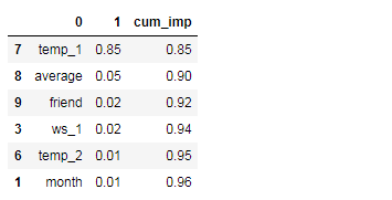
之前是看每个特征的重要性,现在要看特征的累计重要性,先进行排序,再算累计值,用到cunsun()函数,通常以95%为阈值,看多少特征累加在一起之后,其特征重要性的累加值超过该阈值,就取它们作为筛选后的特征。
feature_importances['cum_imp']=np.cumsum(feature_importances.iloc[:,1])
feature_importances.head(6)
做累计特征重要性的图:
plt.figure(figsize=(10,6))
plt.plot(x_values,feature_importances['cum_imp'],'g-')
plt.xticks(x_values,feature_importances.iloc[:,0],rotation='60')
plt.title('cumsum importance')
#添加一条红线
plt.hlines(y=0.95,xmin=0,xmax=len(x_values),color='r',
          linestyles='dashed')

即当第五个特征出现的时候,累计特征重要性超过95%,接下来试着只用这五个特征进行建模,比较一下效果。
建模,只使用重要特征
#看有几个特征
print('num of features for 95% importance:',
     feature_importances[feature_importances['cum_imp']<0.96].shape[0])
num of features for 95% importance: 5
训练模型:
imp_features=feature_importances.iloc[:,0][0:5]

#找到索引在X_test,X_train中对应
imp_indices=[feature_list.index(feature)
            for feature in imp_features]

#训练集和测试集
imp_X_train=X_train[:,imp_indices]
imp_X_test=X_test[:,imp_indices]

#训练模型
fina_rf.fit(imp_X_train,y_train)
查看模型性能:
predictions=fina_rf.predict(imp_X_test)
error=abs(predictions-y_test)
print('平均误差:',round(np.mean(errors),2),'degree.')

mean_mape=round(np.mean(100*error/y_test),2)
print('准确率:',100-mean_mape,'%.')
平均误差: 4.05 degree.
准确率: 93.25 %.
效果还没有上一次好,其实随机森林算法本身会考虑特征的问题,会优先选择有价值的,我们认为的去掉一些,相当于可供候选的少了,出现这样的现象在随机森林中不奇怪。