版权声明:本文为博主原创文章,未经博主允许不得转载。 https://blog.csdn.net/jining11/article/details/88678065
步骤
- 定义拥有一个隐层的神经网络,完成前向和后向传播的算法。(方便起见仅使用weight不使用bias)
- 加载数据并查看其分布。
- 对数据进行一些处理。
- 进行多轮训练。
- 画图并检验预测效果
# 加载必要模块
import numpy as np
import pandas as pd
np.random.seed(1024)
设计每一层的结构
                                   Networks Structure

                                    Input        Weights            Output
Hidden Layer                     [batch_size, 2] x [2,5]   ->   [batch_size, 5]
activation function(sigmoid)     [batch_size, 5]           ->   [batch_size, 5]
Classification Layer             [batch_size, 5] x [5,3]   ->   [batch_size, 3]
activation function(sigmoid)     [batch_size, 3]           ->   [batch_size, 3]
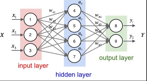
想象一下在下图中,左边是两个神经元,中间五个,右边三个,就和本次情况一样了。
定义神经网络类
class FeedForward_Neural_Network(object):
    def __init__(self, learning_rate):
        # 唯一需要传入的超参数,就是学习率
        self.input_channel = 2
        self.output_channel = 3
        self.hidden_channel = 5
        self.learning_rate = learning_rate
        self.weight1 = np.random.randn(self.input_channel, self.hidden_channel)
        self.weight2 = np.random.randn(self.hidden_channel, self.output_channel)


    def forward(self, X):
        """前向传播,计算真正意义上的矩阵乘积,X的大小是(batch_size*2),o的大小是(batch_size*3)
        """
        self.h1 = np.dot(X, self.weight1)
        self.z1 = self.sigmoid(self.h1)
        self.h2 = np.dot(self.z1, self.weight2)
        o = self.sigmoid(self.h2)
        return o

    def backward(self, X, y, o):
        """后向传播以更新参数,y的值是大小为batch_size*3的one_hot
        """
        # 计算梯度
        # 注意区分*和dot
        self.o_error = y - o
        self.o_delta = self.o_error * self.sigmoid_prime(o)
        self.z1_error = self.o_delta.dot(self.weight2.T)
        self.z1_delta = self.z1_error * self.sigmoid_prime(self.z1)

        # 更新模型参数
        self.weight1 += X.T.dot(self.z1_delta) * self.learning_rate
        self.weight2 += self.z1.T.dot(self.o_delta) * self.learning_rate

    def sigmoid(self, s):
        """激活函数
        """
        return 1 / (1 + np.exp(-s))

    def sigmoid_prime(self, s):
        """激活函数的导数(相对于运算结果来说)
        """
        return s * (1 - s)
-
在每一轮epoch中,将训练集划分为若干个大小为batch size的batch,对每个batch采取如下操作以更新神经网络的参数
- 前向传播,计算输出值。
数学推导:假设每组输入数据包含m个特征即输入向量 包含m个元素,激活函数sigmod用h来表示,输入为b项输出为c项的第a层的权重矩阵用大小为b*c的 来表示,第i层输出结果的第j个分量用 来表示,神经网络共有r层,最终输出结果为R包含m个结果。对于任意矩阵M, 表示其第i行元素构成的向量, 表示第i列元素构成的向量。
有如下推导式:
- 后向回溯,利用链式法则,更新各个参数。
一个关键点是,假设
则
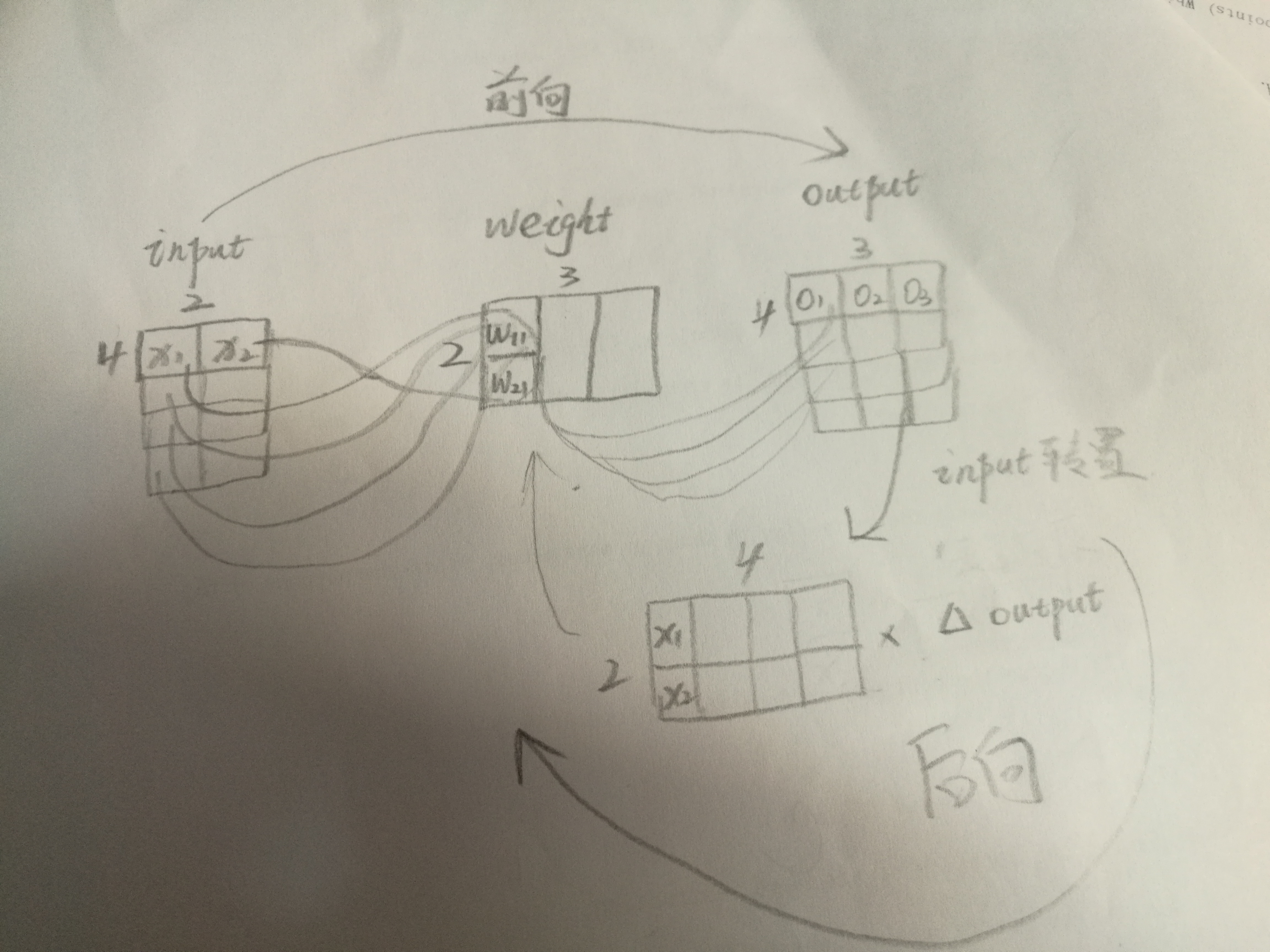
并且, 关于o求导的结果是 ,接下来使用链式求导法则即可。注意到的一点是,某一层的输出矩阵对输入矩阵求导时,矩阵之间求偏导的方式是与输入矩阵的转置相乘。
辅助理解图示:
读取数据
# Import Module
import pandas as pd
import matplotlib.pyplot as plt
import matplotlib.cm as cm
import math
train_csv_file = './labels/train.csv'
test_csv_file = './labels/test.csv'
# Load data from csv file, without header
train_frame = pd.read_csv(train_csv_file, encoding='utf-8', header=None)
test_frame = pd.read_csv(test_csv_file, encoding='utf-8', header=None)
# show data in Dataframe format (defined in pandas)
train_frame[0:5]
| 0 | 1 | 2 | |
|---|---|---|---|
| 0 | 11.834241 | 11.866105 | 1 |
| 1 | 8.101150 | 9.324800 | 1 |
| 2 | 11.184679 | 1.196726 | 2 |
| 3 | 8.911888 | -0.044024 | 2 |
| 4 | 9.863982 | 0.151162 | 2 |
# 区别开特征和标签
train_data = train_frame.iloc[:,0:2].values
train_labels = train_frame.iloc[:,2].values
test_data = test_frame.iloc[:,0:2].values
test_labels = test_frame.iloc[:,2].values
# train & test data shape
print(train_data.shape)
print(test_data.shape)
# train & test labels shape
print(train_labels.shape)
print(test_labels.shape)
(210, 2)
(90, 2)
(210,)
(90,)
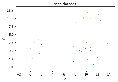
定义绘图函数查看data的空间分布情况
def plot(data, labels, caption):
    # 为每种标签设置不同的颜色,set(labels)可以将标签的所有种类单独提取出来
    colors = cm.rainbow(np.linspace(0, 1, len(set(labels))))
    for i in set(labels):
        xs = []
        ys = []
        # enumerate给labels添加一列递增的索引列
        for index, label in enumerate(labels):
            if label == i:
                xs.append(data[index][0])
                ys.append(data[index][1])
        # 这里这样写是因为labels的值是0,1,2
        plt.scatter(xs, ys, colors[int(i)])
    plt.title(caption)
    plt.xlabel('x')
    plt.ylabel('y')
    plt.show()
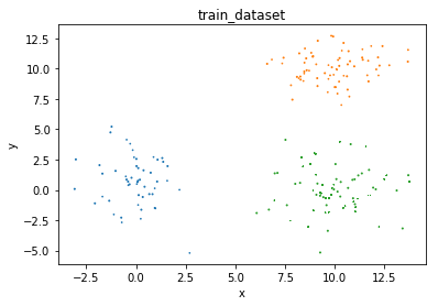
plot(train_data, train_labels, 'train_dataset')
plot(test_data, test_labels, 'test_dataset')
def int2onehot(label):
    """将结果中的label转换成one hot形式
    """
    dims = len(set(label))
    imgs_size = len(label)
    onehot = np.zeros((imgs_size, dims))
    onehot[np.arange(imgs_size), label] = 1
    return onehot
train_labels_onehot = int2onehot(train_labels)
test_labels_onehot = int2onehot(test_labels)
print(train_labels_onehot.shape)
print(train_labels_onehot.shape)
(210, 3)
(210, 3)
def get_accuracy(predictions, labels):
    """predictions是预测值,每组有三个概率值,分别对应着正确结果为三种label中某种的概率大小。labels依然为one-hot的形式。
    """
#     np.argmax()功能为返回数组中最大值的索引
    predictions = np.argmax(predictions, axis=1)
    labels = np.argmax(labels, axis=1)
    all_imgs = len(labels)
#     对布尔类型的矩阵执行np.sum时,false看做0,true看做1
    predict_true = np.sum(predictions == labels)
    return predict_true/all_imgs
def generate_batch(train_data, train_labels, batch_size):
    """生成多个大小为batch_size的batch
    batch_size=len(train_data), GD
    batch_size=1, SGD
    batch_size>1 & batch_size<len(train_data), mini-batch, 如batch_size=2,4,8,16...
    """
    iterations = math.ceil(len(train_data)/batch_size)
    for i in range(iterations):
        index_from = i*batch_size
        index_end = (i+1)*batch_size
#  yield构造生成式,你可能会担心index_end会超出train_data的最大值,但是不要紧,
# 对于有210行的train_data来说,输出train_data[300]当然会报超出范围的错误,
# 但是当中间有个冒号比如[10:300],就会自动对范围进行修正,即使是[300:500]也会输出一个[]
        yield (train_data[index_from:index_end], train_labels[index_from:index_end])
def show_curve(ys, title):
    """绘制损失函数输出值和准确度曲线变化情况
    """
    x = np.array(range(len(ys)))
    y = np.array(ys)
    plt.plot(x, y, c='b')
    plt.axis()
    plt.title('{} Curve:'.format(title))
    plt.xlabel('Epoch')
    plt.ylabel('{} Value'.format(title))
    plt.show()
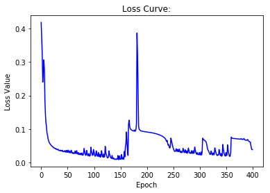
正式开启模型训练,采用GD法
learning_rate = 0.1
epochs = 400 # 使用训练集中全部样本训练的次数
batch_size = len(train_data) # GD
# batch_size = 1               # SGD
# batch_size = 8               # mini-batch
model = FeedForward_Neural_Network(learning_rate) # 初始化神经网络

losses = []
accuracies = []

for i in range(epochs):
    loss = 0
    for index, (xs, ys) in enumerate(generate_batch(train_data, train_labels_onehot, batch_size)):
#         xs是每个batch的input,ys是对应的label
        predictions = model.forward(xs)
        loss += 1/2 * np.mean(np.sum(np.square(ys-predictions), axis=1)) # 将均方差作为损失函数
        model.backward(xs, ys, predictions) # backward phase

    losses.append(loss)
    predictions = model.forward(train_data)
    # 计算准确率
    accuracy = get_accuracy(predictions, train_labels_onehot)
    accuracies.append(accuracy)

    if i % 50 == 0:
        print('Epoch: {}, has {} iterations'.format(i, index+1))
        print('\tLoss: {:.4f}, \tAccuracy: {:.4f}'.format(loss, accuracy))

test_predictions = model.forward(test_data)
# 计算测试集表现
test_accuracy = get_accuracy(test_predictions, test_labels_onehot)
print('Test Accuracy: {:.4f}'.format(test_accuracy))
Epoch: 0, has 1 iterations
	Loss: 0.4625, 	Accuracy: 0.4190
Epoch: 50, has 1 iterations
	Loss: 0.0261, 	Accuracy: 0.9524
Epoch: 100, has 1 iterations
	Loss: 0.2902, 	Accuracy: 0.7095
Epoch: 150, has 1 iterations
	Loss: 0.0118, 	Accuracy: 0.9810
Epoch: 200, has 1 iterations
	Loss: 0.0259, 	Accuracy: 0.9333
Epoch: 250, has 1 iterations
	Loss: 0.0347, 	Accuracy: 0.9714
Epoch: 300, has 1 iterations
	Loss: 0.0312, 	Accuracy: 0.9667
Epoch: 350, has 1 iterations
	Loss: 0.1295, 	Accuracy: 0.8286
Test Accuracy: 0.8444
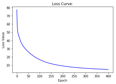
# Draw losses curve using losses
show_curve(losses, 'Loss')
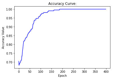
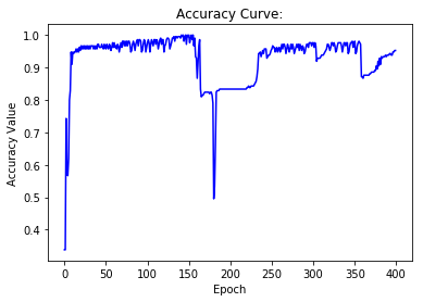
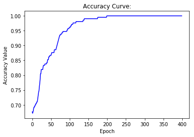
# Draw Accuracy curve using accuracies
show_curve(accuracies, 'Accuracy')
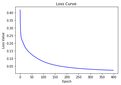
learning rate = 0.01
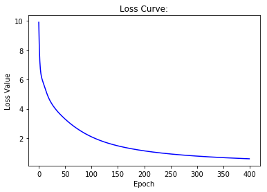
# Draw losses curve using losses
show_curve(losses, 'Loss')
# Draw Accuracy curve using accuracies
show_curve(accuracies, 'Accuracy')
SGD、mini-batch进行比较
# Draw losses curve using losses
show_curve(losses, 'Loss')
# Draw Accuracy curve using accuracies
show_curve(accuracies, 'Accuracy')

# Draw losses curve using losses
show_curve(losses, 'Loss')
# Draw Accuracy curve using accuracies
show_curve(accuracies, 'Accuracy')