
(一)卷积神经网络结构+最终的识别精度。
用Tensorflow实现一个完整的卷积神经网络,用这个卷积神经网络来识别手写数字数据集(MNIST)。我们先来看看实现的卷积神经网络结构如下图所示:

接着,我们再来看看实现的这个卷积神经网络,在MNIST数据集中的测试集上的精度。
我用了两种优化训练方法,对模型训练了1000次,在训练1000的过程中,每隔50次进行一次模型的精度测试。
(1)批量梯度下降法(Batch Gradient Descent),结果如下图所示。学习率为0.001。
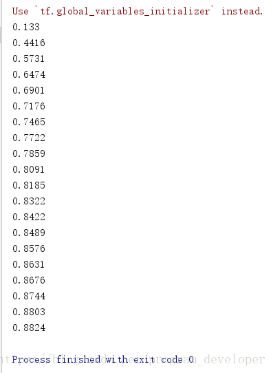
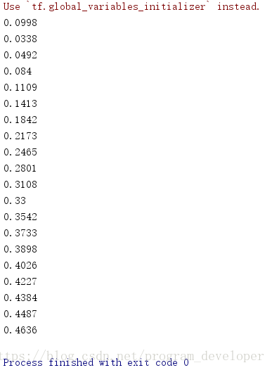
图1:学习率为0.001的批量梯度下降结果 图2:学习率为1e-4的批量梯度下降结果
(2)Adam优化训练方法。结果如下图所示。(学习率为:1e-4也就是1*10^(-4))。

分析两种优化方法的结果:
Adam优化算法比批量梯度下降法更快的到达最优解,使学习器更快的达到最优效果。
(二)实现网络结构
(1)定义卷积层的Weight和bias。
1. 导入Tensorflow模块。
import tensorflow as tf
2. 采用的数据集是Tensorflow里面的mnist数据集。我们需要把数据集导入:
from tensorflow.examples.tutorials.mnist import input_data
# number 1 to 10 data
mnist = input_data.read_data_sets("MNIST_data",one_hot=True)
3. 定义Weight变量,输入shape,返回变量的参数。其中我们使用了tf.truncted_normal产生随机变量来进行初始化:
def weight_variable(shape):
    initial = tf.truncated_normal(shape, stddev=0.1)
    return tf.Variable(initial)
定义biase变量,输入shape,返回变量的一些参数。其中我们使用tf.constant常量函数来进行初始化:
def bias_variable(shape):
    initial = tf.constant(0.1, shape=shape)
    return tf.Variable(initial)
4. 定义卷积操作。tf.nn.conv2d函数是Tensorflow里面的二维的卷积函数,x是图片的所有参数,W是卷积层的权重,然后定义步长strides=[1,1,1,1]值。strides[0]和strides[3]的两个1是默认值,意思是不对样本个数和channel进行卷积,中间两个1代表padding是在x方向运动一步,y方向运动一步,padding采用的方式实“SAME”就是0填充。
def conv2d(x, W):
    # stride[1, x_movement, y_movement, 1]
    # Must have strides[0] = strides[3] =1
    return tf.nn.conv2d(x, W, strides=[1,1,1,1], padding="SAME")  # padding="SAME"用零填充边界
(2)定义池化层
1.定义池化操作。为了得到更多的图片信息,卷积时我们选择的是一次一步,也就是strides[1]=strides[2]=1,这样得到的图片尺寸没有变化,而我们希望压缩一下图片也就是参数能少一些从而减少系统的复杂度,因此我们采用pooling来稀疏化参数,也就是卷积神经网络中所谓的下采样层。pooling有两种,一种是最大值池化,一种是平均值池化,我采用的是最大值池化tf.max_pool()。池化的核函数大小为2*2,因此ksize=[1,2,2,1],步长为2,因此strides=[1,2,2,1]。
def max_pool_2x2(x):
    return tf.nn.max_pool(x, ksize=[1,2,2,1], strides=[1,2,2,1], padding="SAME")
(3)图片输入的处理。
1. 我们定义一下输入的placeholder
# define placeholder for inputs to network
xs = tf.placeholder(tf.float32, [None,784]) # 28*28
ys = tf.placeholder(tf.float32, [None,10])
2.定义dropout的placeholder,它是解决过拟合的有效手段。
# 定义dropout的输入,解决过拟合问题
keep_prob = tf.placeholder(tf.float32)
3. 接着,我们需要处理我们的xs,把xs的形状变成[-1,28,28,1],-1代表先不考虑输入的图片有多少张,后面的1是channel的数量,因为我们输入的图片是黑白的,因此channel是1,如果我们的图片是RGB图像,那么channel就是3。
# 处理xs,把xs的形状变成[-1,28,28,1]
# -1代表先不考虑输入的图片例子多少这个维度。
# 后面的1是channel的数量,因为我们输入的图片是黑白的,因此channel是1。如果是RGB图像,那么channel就是3.
x_image = tf.reshape(xs, [-1, 28, 28, 1])
(4)建立卷积层
1. 我们定义第一层卷积,先定义本层的Weight,本层我们的卷积核大小是5*5,因为黑白图片channel是1,所以输入是1,输出是32个特征图。
W_conv1 = weight_variable([5,5,1,32]) # kernel 5*5, channel is 1, out size 32
2. 定义bias,它的大小是32个长度,因此我们传入它的shape为[32]。
b_conv1 = bias_variable([32])
3. 定义好Weight 和 bias,我们就可以定义卷积神经网络的第一个卷积层h_conv1=conv2d(x_image,W_conv1)+b_conv1,同时我们对h_conv1进行非线性处理,也就是激活函数来处理,这里我们用到的是tf.nn.relu(修正线性单元)来处理,需要注意的是,因为采用了SAME的padding方式,输出图片的大小没有变化依然是28*28,只是厚度变厚了,因此,现在的输出变成了28*28*32。
h_conv1 = tf.nn.relu(conv2d(x_image,W_conv1) + b_conv1) # output size 28*28*32
4. 最后,我们再进行pooling的处理就OK啦!经过pooling的处理,输出大小变成了14*14*32。
h_pool1 = max_pool_2x2(h_conv1) # output size 14*14*32
5. 以同样的方式,我们定义第二个卷积层,本层我们的输入是上面池化层的输出,本层我们的卷积核大小是5*5,有32个特征图,所以输入就是32,输出我们定为64。
W_conv2 = weight_variable([5,5,32,64]) # kernel 5*5, in size 32, out size 64
b_conv2 = bias_variable([64])
6. 接着,我们定义卷积神经网络的第二个卷积层,这时的输出大小就是14*14*64。
h_conv2 = tf.nn.relu(conv2d(h_pool1,W_conv2) + b_conv2) # output size 14*14*64
7. 最后也是一个池化层来处理,输出大小为7*7*64。
h_pool2 = max_pool_2x2(h_conv2) # output size 7*7*64
(5)建立全连接层
1. 我们来定义我们的全连接层。进入全连接层是,我们通过tf.reshape()将h_pool2的输出值从一个三维的变为一个一维的数据,-1表示先不考虑输入图片例子维度,将上一个输出结果展平。
# [n_samples,7,7,64]->>[n_samples, 7*7*64]
h_pool2_flat = tf.reshape(h_pool2, [-1, 7*7*64])
此时,weight_variable的shape输入就是第二个卷积层展平了的输出大小:7*7*64,后面的输出大小我们继续扩大,定为1024。
W_fc1 = weight_variable([7*7*64, 1024])
b_fc1 = bias_variable([1024])
2. 然后,将展平的h_pool2_flat与本层的W_fc1相乘(注意这个时候不是卷积了)。
h_fc1 = tf.nn.relu(tf.matmul(h_pool2_flat, W_fc1) + b_fc1)
3. 我们同时考虑了过拟合的问题,可以加一个dropout的处理。
h_fc1_drop = tf.nn.dropout(h_fc1, keep_prob)
(6)输出层。
1. 我们来构建最后一层:输出层。输入是1024,最后的输出是10(因为mnist数据集就是[0-9]十个类),prediction就是我们最后的预测值。
W_fc2 = weight_variable([1024, 10])
b_fc2 = bias_variable([10])
2. 然后,我们用softmax分类器(多分类,输出的是各个类的概率),对我们的输出进行分类。
prediction = tf.nn.softmax(tf.matmul(h_fc1_drop,W_fc2)+b_fc2)
(7)优化方法。
1. 我们利用交叉熵损失函数来定义我们的cost function。
# the error between prediction and real data
cross_entropy = tf.reduce_mean(-tf.reduce_sum(ys*tf.log(prediction),reduction_indices=[1])) #loss
2. 我们用tf.train.AdamOptimizer()作为我们的优化器进行优化,使我们的cross_entropy最小。
train_step = tf.train.AdamOptimizer(1e-4).minimize(cross_entropy)
当然,也可以用tf.train.GradientDescentOptimizer()作为我们的优化器进行优化。
train_step = tf.train.GradientDescentOptimizer(1e-4).minimize(cross_entropy)
(8)训练
1. 定义session,并初始化所有变量。
sess =tf.Session()
# important step
sess.run(tf.initialize_all_variables())
2. 训练1000次,每个50次检查一下模型的精度。
for i in range(1000):
    batch_xs,batch_ys = mnist.train.next_batch(100)
    sess.run(train_step, feed_dict={xs:batch_xs,ys:batch_ys, keep_prob:0.5})
    if i % 50 ==0:
        # print(sess.run(prediction,feed_dict={xs:batch_xs}))
        print(compute_accuracy(mnist.test.images,mnist.test.labels))
(三)最后,给出完整的代码。
#coding:utf-8
# 导入本次需要的模块
import tensorflow as tf
from tensorflow.examples.tutorials.mnist import input_data
# number 1 to 10 data
mnist = input_data.read_data_sets("MNIST_data",one_hot=True)

def compute_accuracy(v_xs,v_ys):
    global prediction
    y_pre = sess.run(prediction, feed_dict={xs:v_xs, keep_prob:1})
    correct_prediction = tf.equal(tf.argmax(y_pre, 1),tf.argmax(v_ys,1))
    accuracy = tf.reduce_mean(tf.cast(correct_prediction, tf.float32))
    result = sess.run(accuracy, feed_dict={xs:v_xs,ys:v_ys,keep_prob:1})
    return result

def weight_variable(shape):
    initial = tf.truncated_normal(shape, stddev=0.1)
    return tf.Variable(initial)

def bias_variable(shape):
    initial = tf.constant(0.1, shape=shape)
    return tf.Variable(initial)

def conv2d(x, W):
    # stride[1, x_movement, y_movement, 1]
    # Must have strides[0] = strides[3] =1
    return tf.nn.conv2d(x, W, strides=[1,1,1,1], padding="SAME")  # padding="SAME"用零填充边界

def max_pool_2x2(x):
    return tf.nn.max_pool(x, ksize=[1,2,2,1], strides=[1,2,2,1], padding="SAME")

# #################处理图片##################################
# define placeholder for inputs to network
xs = tf.placeholder(tf.float32, [None,784]) # 28*28
ys = tf.placeholder(tf.float32, [None,10])
# 定义dropout的输入,解决过拟合问题
keep_prob = tf.placeholder(tf.float32)
# 处理xs,把xs的形状变成[-1,28,28,1]
# -1代表先不考虑输入的图片例子多少这个维度。
# 后面的1是channel的数量,因为我们输入的图片是黑白的,因此channel是1。如果是RGB图像,那么channel就是3.
x_image = tf.reshape(xs, [-1, 28, 28, 1])
# print(x_image.shape) #[n_samples, 28,28,1]
# #################处理图片##################################

## convl layer ##
W_conv1 = weight_variable([5,5,1,32]) # kernel 5*5, channel is 1, out size 32
b_conv1 = bias_variable([32])
h_conv1 = tf.nn.relu(conv2d(x_image,W_conv1) + b_conv1)  # output size 28*28*32
h_pool1 = max_pool_2x2(h_conv1)                          # output size 14*14*32

## conv2 layer ##
W_conv2 = weight_variable([5,5,32,64]) # kernel 5*5, in size 32, out size 64
b_conv2 = bias_variable([64])
h_conv2 = tf.nn.relu(conv2d(h_pool1,W_conv2) + b_conv2)  # output size 14*14*64
h_pool2 = max_pool_2x2(h_conv2)                          # output size 7*7*64

## funcl layer ##
W_fc1 = weight_variable([7*7*64, 1024])
b_fc1 = bias_variable([1024])

# [n_samples,7,7,64]->>[n_samples, 7*7*64]
h_pool2_flat = tf.reshape(h_pool2, [-1, 7*7*64])
h_fc1 = tf.nn.relu(tf.matmul(h_pool2_flat, W_fc1) + b_fc1)
h_fc1_drop = tf.nn.dropout(h_fc1, keep_prob)

## func2 layer ##
W_fc2 = weight_variable([1024, 10])
b_fc2 = bias_variable([10])
prediction = tf.nn.softmax(tf.matmul(h_fc1_drop,W_fc2)+b_fc2)

# #################优化神经网络##################################
# the error between prediction and real data
cross_entropy = tf.reduce_mean(-tf.reduce_sum(ys*tf.log(prediction),reduction_indices=[1])) #loss
train_step = tf.train.GradientDescentOptimizer(1e-4).minimize(cross_entropy)
# train_step = tf.train.AdamOptimizer(1e-4).minimize(cross_entropy)

sess =tf.Session()
# important step
sess.run(tf.initialize_all_variables())
# #################优化神经网络##################################

for i in range(1000):
    batch_xs,batch_ys = mnist.train.next_batch(100)
    sess.run(train_step, feed_dict={xs:batch_xs,ys:batch_ys, keep_prob:0.5})
    if i % 50 ==0:
        # print(sess.run(prediction,feed_dict={xs:batch_xs}))
        print(compute_accuracy(mnist.test.images,mnist.test.labels))
观看视频笔记:https://morvanzhou.github.io/tutorials/machine-learning/tensorflow/5-05-CNN3/