机器学习：模型评估与优化

版权声明：本文为博主原创文章，未经博主允许不得转载。 https://blog.csdn.net/weixin_40042143/article/details/88285559

Real-World Machine Learning: Model Evaluation and Optimization 

地址：https://livebook.manning.com/#!/book/real-world-machine-learning/chapter-4/9

本文主要是对书上的重要内容进行了提炼翻译笔记，供日后的学习。主要内容包括：

利用交叉验证来评估模型的预测性能

如何避免过拟合

对于二分类和多类别分类的评估指标和可视化

对于回归模型的评估指标和可视化

通过调参来优化模型

---

当你拟合好一个模型后，下一步需要评估这个模型的精确性。在使用模型之前，你应该要了解这个模型对于新的数据的预测能力如何。如果模型的预测性能很好，那么你可以将其用于生产环境中进行数据分析，否则，你需要对你的模型进行优化，提高其准确性。

对ML模型进行性能评估是一件很重要的事情，下面将通过图片和相关的代码给大家展示。

                                                                        图一  ML工作流中的评估与优化

 1.1通用模型：对新数据的预测的准确性评估

对于监督学习的主要目标：预测结果准确。你需要利用训练好的模型对新数据尽可能的预测准确，即模型对新数据的泛化性要好。这样，你的模型应用到生产中才会有好的结果。

1.1.1过拟合问题和模型优化

下面通过一个例子来进行理解：

假设要预测一个农场每亩玉米的产量。你可以通过100个农场的训练数据信息来解决这个回归问题。将每亩的产量和处理过的特征对应绘制如下图，根据图可以看出他们呈现增长性和非线性的关系。

选择一个模型进行训练，可能回出现如下的情况

第一个图：过拟合

第二个图：刚好

第三个图：欠拟合

为了避免过拟合或欠拟和的情况出现，第一步要做的时选择一个 评估指标来刻画的预测性能的好坏。对于回归问题，评估指标均方误差MSE:mean squared error，它是真实值和预测值之间测差值。

注意：不要使用训练模型的数据来评估模型

---

1.1.2交叉验证

问题：训练误差不能很好的指示出模型在新数据上的误差

解决：cross-validation交叉验证CV

常用的两个交叉验证的方法：holdout和k-fold

holdout方法：

将数据集划分成训练集和测试集，训练集用于模型的训练，测试集用于评估模型的准确性。下图展示了holdout方法的一个使用流程。

使用scikit-learn上面关于模型选择的 模块进行holdout方法的实验

import numpy as np
from sklearn.model_selection import train_test_split
from sklearn.metrics import mean_squared_error
from sklearn import datasets
from sklearn import svm

iris = datasets.load_iris()
print(iris.data.shape)
print(iris.target.shape)

# 划分数据集
X_train, X_test, y_train, y_test = train_test_split(iris.data, iris.target, test_size=0.3, random_state=0)

# 训练模型
clf = svm.SVC(kernel='linear', C=1).fit(X_train, y_train)
# 预测
pred_y = clf.predict(X_test)
# 计算MSE
mse = mean_squared_error(y_test, pred_y)
print(mse)

 k-fold方法：

将数据集划分成k个大小相等的互斥子集，每个子集都尽可能的保持一样的数据分布：从数据集中通过分层采样获得。

每次用k-1个子集的并集作为训练集，剩下的那个子集作为测试集--k组训练/测试集。

使用scikit-learn上的模块演示

import numpy as np
from sklearn.model_selection import train_test_split, KFold
from sklearn.metrics import mean_squared_error
from sklearn import datasets
from sklearn import svm

iris = datasets.load_iris()
print(iris.data.shape)
print(iris.target.shape)

mse_arr = []
kf = KFold(n_splits=10)
for train_index, test_index in kf.split(iris.data):
    print("train_index", train_index, "test_index", test_index)
    # 训练模型
    clf = svm.SVC(kernel='linear', C=1).fit(iris.data[train_index], iris.target[train_index])
    # 预测
    pred_y = clf.predict(iris.data[test_index])
    # 计算MSE
    mse = mean_squared_error(iris.target[test_index], pred_y)
 
    mse_arr.append(mse)

print(mse_arr)

使用cross0validation方法时需要注意一下几个问题：

• 划分后的数据集样本分布尽可能一致
• 对于具有时序特征的数据，比如用上个月的收入数据预测这个月的收入数据，在这种情况下，不能出现用未来的数据预测过去的数据的情况
• k值越大，误差估计越好，但是运行时间长----k>=10

---

分类模型的评估

对于二分类问题，测试集标签和预测结果如下图：

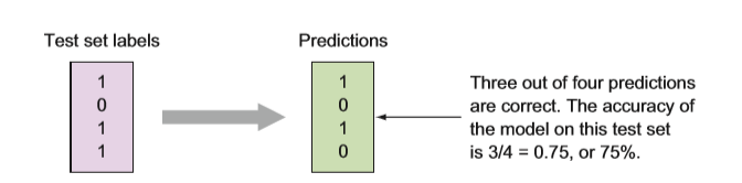
可以看出，有75%的预测结果和真实值一样 

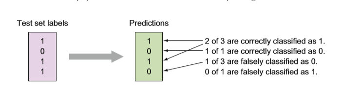
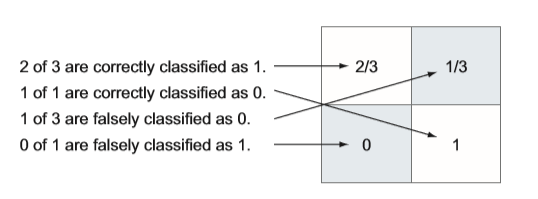
分类结果混淆矩阵

 1.2.2 ROC曲线---可视化工具

对于有一类ML,它的输出是一个实值或者概率，然后将这个预测值和分类阈值进行比较来判别样本的类别。

---概率分类器

ROC曲线通过计算混淆矩阵获得的

二分类ROC曲线（scikit-learn上的例子）

import numpy as np
from scipy import interp
import matplotlib.pyplot as plt

from sklearn import svm, datasets
from sklearn.metrics import roc_curve, auc
from sklearn.model_selection import StratifiedKFold

iris = datasets.load_iris()
features = iris.data
target = iris.target
features, target = features[target != 2], target[target != 2]
n_samples, n_features = features.shape

ramdom_state = np.random.RandomState(0)
features = np.c_[features, ramdom_state.randn(n_samples, 200 * n_features)]

# 分类
cv = StratifiedKFold(n_splits=10)
classifier = svm.SVC(kernel='linear', probability=True, random_state=ramdom_state)

tprs = []
aucs = []
mean_fpr = np.linspace(0, 1, 100)
i = 0
for train, test in cv.split(features, target):
    probas = classifier.fit(features[train], target[train]).predict_proba(features[test])

    # 计算ROC
    """
    roc_curve
    参数：
    y_true:真实值标签（test的标签）
    y_score:预测值概率
    
    返回值：
    fpr:false positive rates
    tpr:true positive rates
    threshold
    """
    fpr, tpr, threshold = roc_curve(target[test], probas[:, 1])
    tprs.append(interp(mean_fpr, fpr, tpr))
    tprs[-1][0] = 0.0
    """
    auc
    参数：
    x:fpr,横坐标
    y:tpr,纵坐标
    return:
    auc:float
    """
    roc_auc = auc(fpr, tpr)
    aucs.append(roc_auc)
    plt.plot(fpr, tpr, lw=1, alpha=0.3,
             label='ROC fold %d (AUC = %0.2f)' % (i, roc_auc))
    i += 1
plt.plot([0, 1], [0, 1], linestyle='--', lw=2, color='r',
         label='Chance', alpha=.8)

mean_tpr = np.mean(tprs, axis=0)
mean_tpr[-1] = 1.0
mean_auc = auc(mean_fpr, mean_tpr)
std_auc = np.std(aucs)
plt.plot(mean_fpr, mean_tpr, color='b',
         label=r'Mean ROC (AUC = %0.2f $\pm$ %0.2f)' % (mean_auc, std_auc),
         lw=2, alpha=.8)

std_tpr = np.std(tprs, axis=0)
tprs_upper = np.minimum(mean_tpr + std_tpr, 1)
tprs_lower = np.maximum(mean_tpr - std_tpr, 0)
plt.fill_between(mean_fpr, tprs_lower, tprs_upper, color='grey', alpha=.2,
                 label=r'$\pm$ 1 std. dev.')

plt.xlim([-0.05, 1.05])
plt.ylim([-0.05, 1.05])
plt.xlabel('False Positive Rate')
plt.ylabel('True Positive Rate')
plt.title('Receiver operating characteristic example')
plt.legend(loc="lower right")
plt.show()

多类别分类ROC曲线（scikit-learn上的例子） 

# 多分类里ROC曲线
import numpy as np
import matplotlib.pyplot as plt
from itertools import cycle

from sklearn import svm, datasets
from sklearn.metrics import roc_curve, auc
from sklearn.model_selection import train_test_split
from sklearn.preprocessing import label_binarize
from sklearn.multiclass import OneVsRestClassifier
from scipy import interp

# Import some data to play with
iris = datasets.load_iris()
X = iris.data
y = iris.target

# Binarize the output
y = label_binarize(y, classes=[0, 1, 2])
n_classes = y.shape[1]

# Add noisy features to make the problem harder
random_state = np.random.RandomState(0)
n_samples, n_features = X.shape
X = np.c_[X, random_state.randn(n_samples, 200 * n_features)]

# 划分训练集和测试集---自定义划分
X_train, X_test, y_train, y_test = train_test_split(X, y, test_size=0.5, random_state=0)

# 利用1:rest策略处理多类别分类任务
classifier = OneVsRestClassifier(svm.SVC(kernel='linear', probability=True, random_state=random_state))

"""
fit:根据训练数据集拟合model
decision_function:计算出决策函数，返回每个类别样本的决策函数
predict(X):预测X类别
score(test_data测试数据,pre_y预测的标签)：mean accuracy
"""
y_score = classifier.fit(X_train, y_train).decision_function(X_test)

# 计算ROC
# Compute ROC curve and ROC area for each class
fpr = dict()
tpr = dict()
roc_auc = dict()
for i in range(n_classes):
    fpr[i], tpr[i], _ = roc_curve(y_test[:, i], y_score[:, i])
    roc_auc[i] = auc(fpr[i], tpr[i])
fpr["micro"], tpr["micro"], _ = roc_curve(y_test.ravel(), y_score.ravel())
roc_auc["mixro"] = auc(fpr["micro"], tpr["micro"])

plt.figure()
lw = 2
plt.plot(fpr[2], tpr[2], color='darkorange', lw=lw, label="ROC cure (area=%0.2f)" % roc_auc[2])
plt.plot([0, 1], [0, 1], color='navy', lw=lw, linestyle='--')
plt.xlim([0.0, 1.0])
plt.ylim([0.0, 1.05])
plt.xlabel('False Positive Rate')
plt.ylabel('True Positive Rate')
plt.title('Receiver operating characteristic example')
plt.legend(loc="lower right")
plt.show()

---

 1.3回归模型的评估

使用交叉验证来评估

对于回归模型来说，回归模型不能通过简单的正确性来评判。一个数值的预测通常情况下不是恰好正确的，它可能回接近或者和正确值相差很大，我们要通过预测值和真实值之间的误差来评估回归模型。

回归模型最简单的一个评估指标：MSE the root mean-square-error和the R-squared value.

MSE:预测值和真实值之间的误差平方和的均值

注意如果实际数据集本身就是很大的数值，那么MSE的计算值可能会很大，这个时候对于模型的评估就没那么好了

所以在计算的时候，可以先将数值型的数据集进行正则化处理，把数值缩小到【0~1】范围内

在使用MSE,RMSE进行回归模型的评估时需要注意：（不怎么理解原文）

---

1.4通过调参来优化模型

1.4.1常见的ML算法和其参数

logistic regression:None

KNN:K,近邻数

Decision Tree:划分指标spliting criterion,树的深度max depth pf tree,划分样本的最小数量minimum samples needed to make a split

Kernel SVM:核函数，核函数的系数，惩罚系数

随机森林：树的数量，每个叶子结点划分特征的数量，划分指标，划分样本的最小数量

Boosting:树的数量，学习率（学习器的权重系数），树的深度，划分指标，划分样本的最小数量

1.4.2grid search

暴力网格搜索；brute-force grid search

将交叉验证和模型评估联系起来

1. 选择评估指标（AUC：分类，MSR or R^2:回归）
2. 选择算法模型
3. 选择要优化的参数以及对应的值放在数组里
4. 将网格定义为参数数组的笛卡儿积
5. 对每个网格里的值，通过交叉验证计算评估指标和预测值
6. 选择评估指标最好的那个模型

scikit-learn上关于网格搜索优化模型的列子

from sklearn import datasets
from sklearn.model_selection import train_test_split
from sklearn.model_selection import GridSearchCV
from sklearn.metrics import classification_report
from sklearn.svm import SVC

print(__doc__)

# Loading the Digits dataset
digits = datasets.load_digits()

# To apply an classifier on this data, we need to flatten the image, to
# turn the data in a (samples, feature) matrix:
n_samples = len(digits.images)
X = digits.images.reshape((n_samples, -1))
y = digits.target

# Split the dataset in two equal parts
X_train, X_test, y_train, y_test = train_test_split(
    X, y, test_size=0.5, random_state=0)

# Set the parameters by cross-validation
tuned_parameters = [{'kernel': ['rbf'], 'gamma': [1e-3, 1e-4],
                     'C': [1, 10, 100, 1000]},
                    {'kernel': ['linear'], 'C': [1, 10, 100, 1000]}]

scores = ['precision', 'recall']
"""
GridSearchVC
参数：
estimator:学习器
param_grid:一个列表，元素是字典类型的，学习器的参数名为key,参数值为value.
scoring:评估指标
cv:使用交叉验证，k
model的属性：
best_estimator:
best_param:

"""
for score in scores:
    print("# Tuning hyper-parameters for %s" % score)
    print()

    clf = GridSearchCV(SVC(), tuned_parameters, cv=5,
                       scoring='%s_macro' % score)
    clf.fit(X_train, y_train)

    print("Best parameters set found on development set:")
    print()
    print(clf.best_params_)
    print()
    print("Grid scores on development set:")
    print()
    means = clf.cv_results_['mean_test_score']
    stds = clf.cv_results_['std_test_score']
    for mean, std, params in zip(means, stds, clf.cv_results_['params']):
        print("%0.3f (+/-%0.03f) for %r"
              % (mean, std * 2, params))
    print()

    print("Detailed classification report:")
    print()
    print("The model is trained on the full development set.")
    print("The scores are computed on the full evaluation set.")
    print()
    y_true, y_pred = y_test, clf.predict(X_test)
    print(classification_report(y_true, y_pred))
    print()