caffe-ssd是一种非常适合新手的end to end 目标识别框架。也是我在学习了深度学习和目标识别理论以后第一个上手跑的程序。具体步骤如下:
一 SSD的安装
- 下载caffe,如果没有配置过可以参考:https://blog.csdn.net/baobei0112/article/details/77996369
- 在home目录下,获取SSD的代码,下载完成后有一个caffe文件夹
 1  git clone https://github.com/weiliu89/caffe.git
 2  cd caffe
 3  git checkout ssd(出现“分支”则说明copy-check成功)
- 进入下载好的caffe目录,复制配置文件
  1     cd /home/usrname/caffe
2 cp Makefile.config.example Makefile.config 3 然后修改Makefile.config,照之前caffe文件下修改即可- 编译caffe
1 make all -j4
2 make test
3 make runtest
- 编译Python wrapper
make pycaffe
不报错说明成功。

二 数据集的准备
- 准备好标注好的图片数据
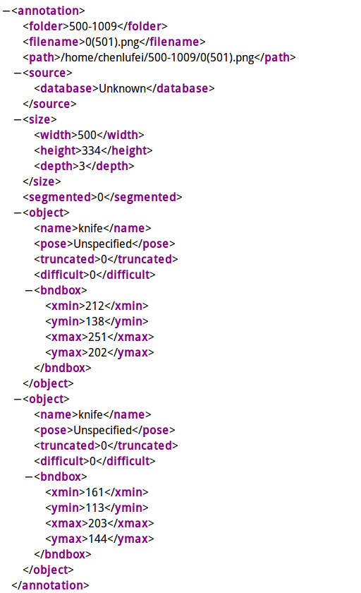
- 我是用labelImage(使用方法自行百度)来标注图片,标注好的图片会有与其名称对应的xml文件保存识别框位置,具体如下:
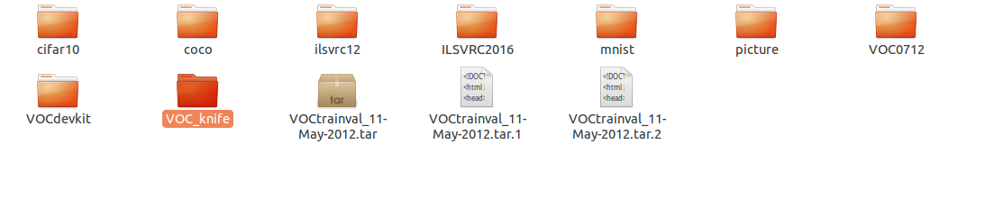
- 在data文件夹下新建自己训练数据的VOC格式文件(VOC_knife):
- 在voc文件夹下新建4个文件夹:
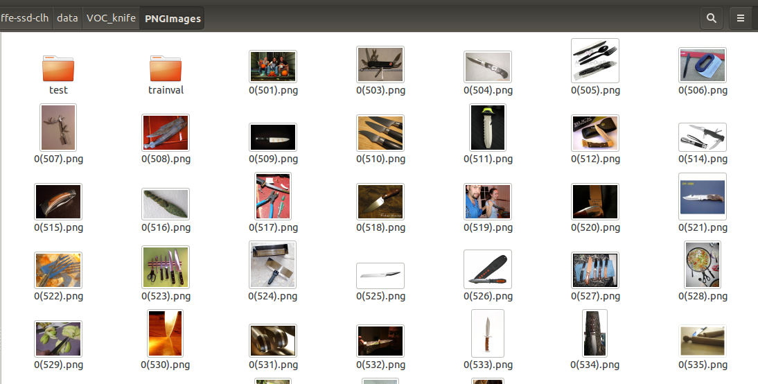
- 将标注好的所有xml文件放入Annotations中,将所有图片放入PNGImages中。
- 在PNGImages新建两个文件夹trainval和test,将PNGImages中的图片按4:1(具体多少不一定,我是这么分的)放入trainval和test中(也就是说所有图片在PNGImages中有,在trainval和test中还有一份,如此是为了方便接下来脚本方便生成数据集):
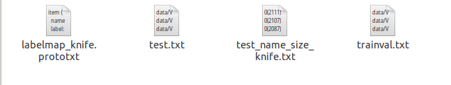
- 在ImageSets中应有如下4个txt文档:
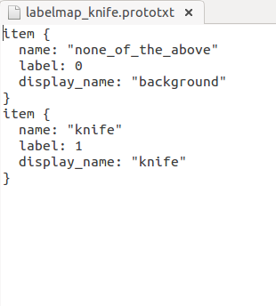
- 首先是labelmap.prototxt按实际项目写成如下格式,若有多个分类依次往下手动编写即可,需要注意的是都需要编写背景类0:
- 其次是trainval和test两个txt文本,用如下脚本编写即可,只需改变脚本中相应图片与xml文件的路径便可生成:
- #! /usr/bin/python
# -*- coding:UTF-8 -*-
import os, sys
import glob
#训练集和测试集路径
trainval_dir = "/home/u809-1/caffe-ssd-clh/data/VOC_knife/PNGImages/trainval"
test_dir = "/home/u809-1/caffe-ssd-clh/data/VOC_knife/PNGImages/test"
trainval_img_lists = glob.glob(trainval_dir + '/*.png') #获取trainval中所有.png的文件
trainval_img_names = [] #获取名称
for item in trainval_img_lists:
temp1, temp2 = os.path.splitext(os.path.basename(item))
trainval_img_names.append(temp1)
test_img_lists = glob.glob(test_dir + '/*.png') #获取test中所有.png文件
test_img_names = []
for item in test_img_lists:
temp1, temp2 = os.path.splitext(os.path.basename(item))
test_img_names.append(temp1)
#图片路径和xml路径
dist_img_dir = "data/VOC_knife/PNGImages" #需要写入txt的trainval和test路径,因为我们在PNGImges目录下除了有trainval和test文件夹外还有所有图片,所以只用写到PNGImages
dist_anno_dir = "/data/VOC_knife/Annotations" #需要写入的xml路径 !!!从caffe跟目录下第一个文件开始写
trainval_fd = open("/home/u809-1/caffe-ssd-clh/data/VOC_knife/ImageSets/trainval.txt", 'w') #存到哪里,及存储的名称
test_fd = open("/home/u809-1/caffe-ssd-clh/data/VOC_knife/ImageSets/test.txt", 'w')
for item in trainval_img_names:
trainval_fd.write(dist_img_dir + '/' + str(item) + '.png' + ' ' + dist_anno_dir + '/' + str(item) + '.xml\n')
for item in test_img_names:
test_fd.write(dist_img_dir + '/' + str(item) + '.png' + ' ' + dist_anno_dir + '/' + str(item) + '.xml\n') - 最后是test_name_size.txt文档,同样用脚本生成:
- #! /usr/bin/python
# -*- coding:UTF-8 -*-
import os, sys
import glob
from PIL import Image #读图
#图的路径
img_dir = "/home/u809-1/caffe-ssd-clh/data/VOC_knife/PNGImages/test"
#获取制定路径下的所有png图片的名称
img_lists = glob.glob(img_dir + '/*.png')
#在指定路径下创建文件
test_name_size = open('/home/u809-1/caffe-ssd-clh/data/VOC_knife/test_name_size_knife.txt', 'w')
for item in img_lists:
img = Image.open(item)
width, height = img.size
temp1, temp2 = os.path.splitext(os.path.basename(item))
test_name_size.write(temp1 + ' ' + str(height) + ' ' + str(width) + '\n') - 这时已经准备好VOC格式的数据了,最后一步将VOC转换成LMDB格式的数据就可以用作训练了:
- cur_dir=$(cd $( dirname ${BASH_SOURCE[0]} ) && pwd )
root_dir='/home/u809-1/caffe-ssd-clh'
cd $root_dir
redo=1
data_root_dir="$HOME/caffe-ssd-clh"
dataset_name="VOC_knife/ImageSets" #上下相连到最终VOC
mapfile="/home/u809-1/caffe-ssd-clh/data/VOC_knife/ImageSets/labelmap_knife.prototxt" #次文件定义了背景层0,以及分类层,下次直接定义labelmap.prototxt的直接路径即可
anno_type="detection"
db="lmdb"
min_dim=0
max_dim=0
width=0
height=0
extra_cmd="--encode-type=png --encoded"
if [ $redo ]
then
extra_cmd="$extra_cmd --redo"
fi
for subset in test trainval
do #下面的路径需要根据自己的情况修改,我们的就是这样
python $root_dir/scripts/create_annoset.py --anno-type=$anno_type --label-map-file=$mapfile --min-dim=$min_dim --max-dim=$max_dim --resize-width=$width --resize-height=$height --check-label $extra_cmd $data_root_dir $root_dir/data/$dataset_name/$subset.txt $data_root_dir/$dataset_name/$db/$dataset_name"_"$subset"_"$db examples/$dataset_name
done - 需要注意这个脚本是shell脚本,修改路径时请仔细修改。
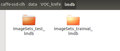
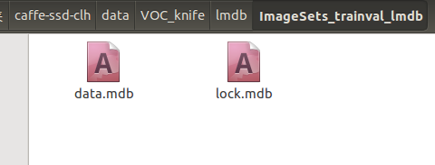
- 生成后的lmdb如下:
- 此时lmdb格式数据集合已经准备完了,开始训练!
三 训练自己的caffe.model
- 用如下脚本进行训练,需修改路径和其中solver.prototxt:
- from __future__ import print_function
import caffe
from caffe.model_libs import *
from google.protobuf import text_format
import math
import os
import shutil
import stat
import subprocess
import sys
# 给基准网络后面增加额外的卷积层(为了避免此处的卷积层的名称和基准网络卷积层的名称重复,这里可以用基准网络最后一个层的名称进行开始命名),这一部分的具体实现方法可以对照文件~/caffe/python/caffe/model_libs.py查看,SSD的实现基本上就是ssd_pascal.py和model_libs.py两个文件在控制,剩下的则是caffe底层代码中编写各个功能模块。
def AddExtraLayers(net, use_batchnorm=True, lr_mult=1):
use_relu = True
# Add additional convolutional layers.
# 19 x 19
######################################生成附加网络的第一个卷积层,卷积核的数量为256,卷积核的大小为1*1,pad的尺寸为0,stride为1.
from_layer = net.keys()[-1] #获得基准网络的最后一层,作为conv6-1层的输入
# TODO(weiliu89): Construct the name using the last layer to avoid duplication.
# 10 x 10
out_layer = "conv6_1"
ConvBNLayer(net, from_layer, out_layer, use_batchnorm, use_relu, 256, 1, 0, 1,
lr_mult=lr_mult)
########################################conv6_1生成完毕
######################################生成附加网络的第一个卷积层,卷积核的数量为512,卷积核的大小为3*3,pad的尺寸为1,stride为2.
from_layer = out_layer
out_layer = "conv6_2"
ConvBNLayer(net, from_layer, out_layer, use_batchnorm, use_relu, 512, 3, 1, 2,
lr_mult=lr_mult)
#########################################conv6_2生成完毕
# 5 x 5
from_layer = out_layer
out_layer = "conv7_1"
ConvBNLayer(net, from_layer, out_layer, use_batchnorm, use_relu, 128, 1, 0, 1,
lr_mult=lr_mult)
#########################################conv7_1生成完毕
from_layer = out_layer
out_layer = "conv7_2"
ConvBNLayer(net, from_layer, out_layer, use_batchnorm, use_relu, 256, 3, 1, 2,
lr_mult=lr_mult)
#########################################conv7_2生成完毕
# 3 x 3
from_layer = out_layer
out_layer = "conv8_1"
ConvBNLayer(net, from_layer, out_layer, use_batchnorm, use_relu, 128, 1, 0, 1,
lr_mult=lr_mult)
#########################################conv8_1生成完毕
from_layer = out_layer
out_layer = "conv8_2"
ConvBNLayer(net, from_layer, out_layer, use_batchnorm, use_relu, 256, 3, 0, 1,
lr_mult=lr_mult)
#########################################conv8_2生成完毕
# 1 x 1
from_layer = out_layer
out_layer = "conv9_1"
ConvBNLayer(net, from_layer, out_layer, use_batchnorm, use_relu, 128, 1, 0, 1,
lr_mult=lr_mult)
#########################################conv9_1生成完毕
from_layer = out_layer
out_layer = "conv9_2"
ConvBNLayer(net, from_layer, out_layer, use_batchnorm, use_relu, 256, 3, 0, 1,
lr_mult=lr_mult)
#########################################conv9_2生成完毕
return net
### 相应地修改一下参数 ###
# 包含caffe代码的路径
# 我们假设你是在caffe跟目录下运行代码
caffe_root = os.getcwd() #获取caffe的根目录
# 如果你想在生成所有训练文件之后就开始训练,这里run_soon给予参数Ture.
run_soon = True
#如果你想接着上次的训练,继续进行训练,这里的参数为Ture,(这个就是说可能你训练一般停止了,重新启动的时候,这里的Ture保证继续接着你上次的训练进行训练)
#否则为False,表示我们将从下面定义的预训练模型处进行加载。(这个表示就是不管你上次训练一半的模型了,我们直接从预训练好的基准模型哪里开始训练)
resume_training = True
# 如果是Ture的话,表示我们要移除旧的模型训练文件,否则是不移除的。
remove_old_models = False
# 训练数据的数据库文件. Created by data/VOC0712/create_data.sh
train_data = "examples/VOC0712/VOC0712_trainval_lmdb"
# 测试数据的数据库文件. Created by data/VOC0712/create_data.sh
test_data = "examples/VOC0712/VOC0712_test_lmdb"
# 指定批量采样器。
resize_width = 300
resize_height = 300
resize = "{}x{}".format(resize_width, resize_height)
batch_sampler = [
{
'sampler': {
},
'max_trials': 1,
'max_sample': 1,
},
{
'sampler': {
'min_scale': 0.3,
'max_scale': 1.0,
'min_aspect_ratio': 0.5,
'max_aspect_ratio': 2.0,
},
'sample_constraint': {
'min_jaccard_overlap': 0.1,
},
'max_trials': 50,
'max_sample': 1,
},
{
'sampler': {
'min_scale': 0.3,
'max_scale': 1.0,
'min_aspect_ratio': 0.5,
'max_aspect_ratio': 2.0,
},
'sample_constraint': {
'min_jaccard_overlap': 0.3,
},
'max_trials': 50,
'max_sample': 1,
},
{
'sampler': {
'min_scale': 0.3,
'max_scale': 1.0,
'min_aspect_ratio': 0.5,
'max_aspect_ratio': 2.0,
},
'sample_constraint': {
'min_jaccard_overlap': 0.5,
},
'max_trials': 50,
'max_sample': 1,
},
{
'sampler': {
'min_scale': 0.3,
'max_scale': 1.0,
'min_aspect_ratio': 0.5,
'max_aspect_ratio': 2.0,
},
'sample_constraint': {
'min_jaccard_overlap': 0.7,
},
'max_trials': 50,
'max_sample': 1,
},
{
'sampler': {
'min_scale': 0.3,
'max_scale': 1.0,
'min_aspect_ratio': 0.5,
'max_aspect_ratio': 2.0,
},
'sample_constraint': {
'min_jaccard_overlap': 0.9,
},
'max_trials': 50,
'max_sample': 1,
},
{
'sampler': {
'min_scale': 0.3,
'max_scale': 1.0,
'min_aspect_ratio': 0.5,
'max_aspect_ratio': 2.0,
},
'sample_constraint': {
'max_jaccard_overlap': 1.0,
},
'max_trials': 50,
'max_sample': 1,
},
]
#以上这一部分就是文中所说的数据增强部分,抱歉的是这一部分我也没太看懂。具体可查看~/caffe/src/caffe/util/sampler.cpp文件中的详细定义。
#以下是转换参数设置,具体意思可在caffe底层代码中查看参数的定义。路径为~/caffe/src/caffe/proto/caffe.proto
train_transform_param = {
'mirror': True,
'mean_value': [104, 117, 123],############均值
'resize_param': { #################存储数据转换器用于调整大小策略的参数的消息。
'prob': 1, ###############使用这个调整策略的可能性
'resize_mode': P.Resize.WARP, ########重定义大小的模式,caffe.proto中定义的是枚举类型
'height': resize_height,
'width': resize_width,
'interp_mode': [ ###########插值模式用于调整大小,定义为枚举类型
P.Resize.LINEAR,
P.Resize.AREA,
P.Resize.NEAREST,
P.Resize.CUBIC,
P.Resize.LANCZOS4,
],
},
'distort_param': {##########################存储数据转换器用于失真策略的参数的消息
'brightness_prob': 0.5, ###########调整亮度的概率,默认为1。
'brightness_delta': 32, ###########要添加到[-delta,delta]内的像素值的数量。可能的值在[0,255]之内。 推荐32。
'contrast_prob': 0.5, #######调整对比度的概率。
'contrast_lower': 0.5, #######随机对比因子的下界。 推荐0.5。
'contrast_upper': 1.5, #######随机对比因子的上界。 推荐1.5。
'hue_prob': 0.5, ##########调整色调的概率。
'hue_delta': 18, ##########添加到[-delta,delta]内的色调通道的数量。 可能的值在[0,180]之内。 推荐36。
'saturation_prob': 0.5, ########调整饱和的概率。
'saturation_lower': 0.5, ########随机饱和因子的下界。 推荐0.5。
'saturation_upper': 1.5, ########随机饱和因子的上界。 推荐1.5。
'random_order_prob': 0.0, ########随机排列图像通道的概率。
},
'expand_param': { ##################存储数据转换器用于扩展策略的参数的消息
'prob': 0.5, ###############使用这个扩展策略的可能性
'max_expand_ratio': 4.0, ######扩大图像的比例。
},
'emit_constraint': { ########给定注释的条件。
'emit_type': caffe_pb2.EmitConstraint.CENTER, ##############类型定义为枚举,此处选定为CENTER
}
}
test_transform_param = { ###############测试转换参数,类似于训练转换参数。
'mean_value': [104, 117, 123],
'resize_param': {
'prob': 1,
'resize_mode': P.Resize.WARP,
'height': resize_height,
'width': resize_width,
'interp_mode': [P.Resize.LINEAR],
},
}
# 如果为true,则对所有新添加的图层使用批量标准。
# 目前只有非批量规范版本已经过测试。
use_batchnorm = False ###############是否使用批量标准
lr_mult = 1 #############基础学习率设定为1,用于下面的计算以改变初始学习率。
# 使用不同的初始学习率。
if use_batchnorm:
base_lr = 0.0004
else:
# 当batch_size = 1, num_gpus = 1时的学习率。
base_lr = 0.00004 ############由于上面use_batchnorm = false,所以我们一般调整初始学习率时只需更改这一部分,目前为0.001。
#你改你的model
# Modify the job name if you want.
job_name = "SSD_{}".format(resize)
# The name of the model. Modify it if you want.
model_name = "VGG_VOC0712_{}".format(job_name)
#存储模型.prototxt文件的目录。
save_dir = "models/VGGNet/VOC0712/{}".format(job_name)
# 存储模型快照的目录。
snapshot_dir = "models/VGGNet/VOC0712/{}".format(job_name)
# 存储作业脚本和日志文件的目录。
job_dir = "jobs/VGGNet/VOC0712/{}".format(job_name)
# 存储检测结果的目录。
output_result_dir = "{}/data/VOCdevkit/results/VOC2007/{}/Main".format(os.environ['HOME'], job_name)
# 模型定义文件。
train_net_file = "{}/train.prototxt".format(save_dir)
test_net_file = "{}/test.prototxt".format(save_dir)
deploy_net_file = "{}/deploy.prototxt".format(save_dir)
solver_file = "{}/solver.prototxt".format(save_dir)
# 快照前缀。
snapshot_prefix = "{}/{}".format(snapshot_dir, model_name)
# 作业脚本路径。
job_file = "{}/{}.sh".format(job_dir, model_name)
# 存储测试图像的名称和大小。 Created by data/VOC0712/create_list.sh
name_size_file = "data/VOC0712/test_name_size.txt"
# 预训练模型。 我们使用完卷积截断的VGGNet。
pretrain_model = "models/VGGNet/VGG_ILSVRC_16_layers_fc_reduced.caffemodel"
# 存储LabelMapItem。
label_map_file = "data/VOC0712/labelmap_voc.prototxt"
# 多框损失层MultiBoxLoss的参数。在~/caffe/src/caffe/proto/caffe.proto可查找具体定义
num_classes = 21 ##########要预测的类的数量。你的分类数+1
share_location = True #########位置共享,如果为true,边框在不同的类中共享。
background_label_id=0 ########是否使用先验匹配,一般为true。
train_on_diff_gt = True ########是否考虑困难的ground truth,默认为true。
normalization_mode = P.Loss.VALID ######如何规范跨越批次,空间维度或其他维度聚集的损失层的损失。 目前只在SoftmaxWithLoss和SigmoidCrossEntropyLoss图层中实现。按照批次中的示例数量乘以空间维度。 在计算归一化因子时,不会忽略接收忽略标签的输出。定义为枚举,四种类型分别是:FULL,除以不带ignore_label的输出位置总数。 如果未设置ignore_label,则表现为FULL;VALID;BATCH_SIZE,除以批量大小;NONE,不要规范化损失。
code_type = P.PriorBox.CENTER_SIZE #########bbox的编码方式。此参数定义在PriorBoxParameter参数定义解释中,为枚举类型,三种类型为:CORNER,CENTER_SIZE和CORNER_SIZE。
ignore_cross_boundary_bbox = False ########如果为true,则在匹配期间忽略跨边界bbox。 跨界bbox是一个在图像区域之外的bbox。即将超出图像的预测边框剔除,这里我们不踢除,否则特征图边界点产生的先验框就没有任何意义。
mining_type = P.MultiBoxLoss.MAX_NEGATIVE 训练期间的挖掘类型。定义为枚举,分别为三种类型: 若为NONE则表示什么都不使用,这样会导致正负样本的严重不均衡;若为MAX_NEGATIVE则根据分数选择底片;若为HARD_EXAMPLE则选择基于“在线硬示例挖掘的基于训练区域的对象探测器”的硬实例,此类型即为SSD原文中所使用的Hard_negative_mining(负硬挖掘)策略。
neg_pos_ratio = 3. #####负/正比率,即文中所说的1:3。
loc_weight = (neg_pos_ratio + 1.) / 4. #########位置损失的权重,
multibox_loss_param = { ############存储MultiBoxLossLayer使用的参数的消息
'loc_loss_type': P.MultiBoxLoss.SMOOTH_L1, ###########位置损失类型,定义为枚举,有L2和SMOOTH_L1两种类型。
'conf_loss_type': P.MultiBoxLoss.SOFTMAX, #########置信损失类型,定义为枚举,有SOFTMAX和LOGISTIC两种。
'loc_weight': loc_weight,
'num_classes': num_classes,
'share_location': share_location,
'match_type': P.MultiBoxLoss.PER_PREDICTION, #########训练中的匹配方法。定义为枚举,有BIPARTITE和PER_PREDICTION两种。如果match_type为PER_PREDICTION(即每张图预测),则使用overlap_threshold来确定额外的匹配bbox。
'overlap_threshold': 0.5, #########阀值大小。即我们所说的IoU的大小。
'use_prior_for_matching': True, ########是否使用先验匹配,一般为true。
'background_label_id': background_label_id, ##########背景标签的类别编号,一般为0。
'use_difficult_gt': train_on_diff_gt, ########是否考虑困难的ground truth,默认为true。
'mining_type': mining_type, #######训练期间的挖掘类型。定义为枚举,分别为三种类型: 若为NONE则表示什么都不使用,这样会导致正负样本的严重不均衡;若为MAX_NEGATIVE则根据分数选择底片;若为HARD_EXAMPLE则选择基于“在线硬示例挖掘的基于训练区域的对象探测器”的硬实例,此类型即为SSD原文中所使用的Hard_negative_mining(负硬挖掘)策略。
'neg_pos_ratio': neg_pos_ratio, #####负/正比率,即文中所说的1:3。
'neg_overlap': 0.5, ####对于不匹配的预测,上限为负的重叠。即如果重叠小于0.5则定义为负样本,Faster R-CNN设置为0.3。
'code_type': code_type, #########bbox的编码方式。此参数定义在PriorBoxParameter参数定义解释中,为枚举类型,三种类型为:CORNER,CENTER_SIZE和CORNER_SIZE。
'ignore_cross_boundary_bbox': ignore_cross_boundary_bbox, ########如果为true,则在匹配期间忽略跨边界bbox。 跨界bbox是一个在图像区域之外的bbox。即将超出图像的预测边框剔除,这里我们不踢除,否则特征图边界点产生的先验框就没有任何意义。
}
loss_param = { ###存储由损失层共享的参数的消息
'normalization': normalization_mode, ######如何规范跨越批次,空间维度或其他维度聚集的损失层的损失。 目前只在SoftmaxWithLoss和SigmoidCrossEntropyLoss图层中实现。按照批次中的示例数量乘以空间维度。 在计算归一化因子时,不会忽略接收忽略标签的输出。定义为枚举,四种类型分别是:FULL,除以不带ignore_label的输出位置总数。 如果未设置ignore_label,则表现为FULL;VALID;BATCH_SIZE,除以批量大小;NONE,不要规范化损失。
}
#参数生成先验。
#输入图像的最小尺寸
min_dim = 300 #######维度
# conv4_3 ==> 38 x 38
# fc7 ==> 19 x 19
# conv6_2 ==> 10 x 10
# conv7_2 ==> 5 x 5
# conv8_2 ==> 3 x 3
# conv9_2 ==> 1 x 1
mbox_source_layers = ['conv4_3', 'fc7', 'conv6_2', 'conv7_2', 'conv8_2', 'conv9_2'] #####prior_box来源层,可以更改。很多改进都是基于此处的调整。
# in percent %
min_ratio = 20 ####这里即是论文中所说的Smin=0.2,Smax=0.9的初始值,经过下面的运算即可得到min_sizes,max_sizes。具体如何计算以及两者代表什么,请关注我的博客SSD详解。这里产生很多改进。
max_ratio = 90
####math.floor()函数表示:求一个最接近它的整数,它的值小于或等于这个浮点数。
step = int(math.floor((max_ratio - min_ratio) / (len(mbox_source_layers) - 2)))####取一个间距步长,即在下面for循环给ratio取值时起一个间距作用。可以用一个具体的数值代替,这里等于17。
min_sizes = [] ###经过以下运算得到min_sizes和max_sizes。
max_sizes = []
for ratio in xrange(min_ratio, max_ratio + 1, step): ####从min_ratio至max_ratio+1每隔step=17取一个值赋值给ratio。注意xrange函数的作用。
########min_sizes.append()函数即把括号内部每次得到的值依次给了min_sizes。
min_sizes.append(min_dim * ratio / 100.)
max_sizes.append(min_dim * (ratio + step) / 100.)
min_sizes = [min_dim * 10 / 100.] + min_sizes
max_sizes = [min_dim * 20 / 100.] + max_sizes
steps = [8, 16, 32, 64, 100, 300] ###这一步要仔细理解,即计算卷积层产生的prior_box距离原图的步长,先验框中心点的坐标会乘以step,相当于从feature map位置映射回原图位置,比如conv4_3输出特征图大小为38*38,而输入的图片为300*300,所以38*8约等于300,所以映射步长为8。这是针对300*300的训练图片。
aspect_ratios = [[2], [2, 3], [2, 3], [2, 3], [2], [2]] #######这里指的是横纵比,六种尺度对应六个产生prior_box的卷积层。具体可查看生成的train.prototxt文件一一对应每层的aspect_ratio参数,此参数在caffe.proto中有定义,关于aspect_ratios如何把其内容传递给了aspect_ratio,在model_libs.py文件中有详细定义。
##在此我们要说明一个事实,就是文中的长宽比是如何产生的,这里请读者一定要参看博主博文《SSD详解(一)》中的第2部分内容,关于prior_box的产生。
# L2 normalize conv4_3.
normalizations = [20, -1, -1, -1, -1, -1] ##对卷积层conv4_3做归一化。model_libs.py里产生了normallize层,具体的层定义,参看底层代码~/caffe/src/layers/Normalize_layer.cpp,为什么这里设置conv4_3为20我也没看懂,原谅C++太渣,这里每个数对应每个先验层,只要哪个层对应的数不为-1则产生normal。
# 用于对之前的bbox进行编码/解码的方差。
if code_type == P.PriorBox.CENTER_SIZE: ########两种选择,根据参数code_type的选择决定,由于上面已经将code_type选定。有人理解为变量variance用来对bbox的回归目标进行放大,从而加快对应滤波器参数的收敛。除以variance是对预测box和真实box的误差进行放大,从而增加loss,增大梯度,加快收敛。另外,top_data += top[0]->offset(0, 1);已经使指针指向新的地址,所以variance不会覆盖前面的结果。prior_variance在model_libs.py中传递给了variance变量,然后利用prior_box_layer.cpp将其运算定义至priorbox_layer层中,具体可查看train.prototxt中的每一个先验卷积层层中产生先验框的层中,即**_mbox_priorbox。
prior_variance = [0.1, 0.1, 0.2, 0.2]
else:
prior_variance = [0.1]
flip = True ###如果为true,则会翻转每个宽高比。例如,如果有纵横比“r”,我们也会产生纵横比“1.0 / r”。故产生{1,2,3,1/2,1/3}。
clip = False ###做clip操作是为了让prior的候选坐标位置保持在[0,1]范围内。在caffe.proto文件中有关于参数clip的解释,为”如果为true,则将先验框裁剪为[0,1]“。
#以上两个参数所产生的结果均在prior_box_layer.cpp中实现。
# 求解参数。
# 定义要使用的GPU。
gpus = "0,1,2,3" #多块GPU的编号,如果只有一块,这里只需保留0,否则会出错。
gpulist = gpus.split(",") #获取GPU的列表。
num_gpus = len(gpulist) #获取GPU编号。
# 将小批量分成不同的GPU.
batch_size = 32 #设置训练样本输入的数量,不要超出内存就好。
accum_batch_size = 32 #这里与batch_size相搭配产生下面的iter_size。在看了下一行你就知道它的作用了。
iter_size = accum_batch_size / batch_size #如果iter_size=1,则前向传播一次后进行一次反向传递,如果=2,则两次前传后进行一次反传,这样做是减少每次传播所占用的内存空间,有的硬件不行的话就无法训练,但是增加iter会使训练时间增加,但是总的迭代次数不变。
solver_mode = P.Solver.CPU
device_id = 0
batch_size_per_device = batch_size #批次传递,没什么好讲的。
if num_gpus > 0:
batch_size_per_device = int(math.ceil(float(batch_size) / num_gpus)) #这里指如果你有多块GPU则可以将这些训练任务均分给多块GPU训练,从而加快训练速度。
iter_size = int(math.ceil(float(accum_batch_size) / (batch_size_per_device * num_gpus))) #多块GPU的iter_size大小计算,上面的是一块的时候。
solver_mode = P.Solver.GPU
device_id = int(gpulist[0])
if normalization_mode == P.Loss.NONE: ##如果损失层的参数NormalizationMode选择NONE,即没有归一化模式,则基础学习率为本文件之上的base_lr=0.0004除以batch_size_per_device=32得到新的base_lr=1.25*10^(-5)。
base_lr /= batch_size_per_device
elif normalization_mode == P.Loss.VALID: ##同理,根据不同的归一化模式选择不同的base_lr。在本文件上面我们看到了normalization_mode = P.Loss.VALID,而loc_weight = (neg_pos_ratio + 1.) / 4==1,所以新的base_lr=25*0.0004=0.001,这就是为什么我们最后生成的solver.prototxt文件中的base_lr=0.001的原因,所以如果训练发散想通过减小base_lr来实验,则要更改最上面的base_lr=0.0004才可以。
base_lr *= 25. / loc_weight
elif normalization_mode == P.Loss.FULL: #同上理。
# 每幅图像大概有2000个先验bbox。
# TODO(weiliu89): 估计确切的先验数量。
base_lr *= 2000. #base_lr=2000*0.0004=0.8。
# 评估整个测试集。
num_test_image = 4952 #整个测试集图像的数量。
test_batch_size = 8 #测试时的batch_size。
# 理想情况下,test_batch_size应该被num_test_image整除,否则mAP会略微偏离真实值。
test_iter = int(math.ceil(float(num_test_image) / test_batch_size)) #这里计算每测试迭代多少次可以覆盖整个测试集,和分类网络中的是一致的。这里4952/8=619,如果你的测试图片除以你的test_batch_size不等于整数,那么这里会取一个近似整数。
solver_param = { ##solver.prototxt文件中的各参数的取值,这里相信做过caffe训练的人应该大致有了解。
# 训练参数
'base_lr': base_lr, #把上面的solver拿下来。
'weight_decay': 0.0005,
'lr_policy': "multistep",
'stepvalue': [80000, 100000, 120000], #多步衰减
'gamma': 0.1,
'momentum': 0.9,
'iter_size': iter_size,
'max_iter': 120000,
'snapshot': 80000,
'display': 10,
'average_loss': 10,
'type': "SGD",
'solver_mode': solver_mode,
'device_id': device_id,
'debug_info': False,
'snapshot_after_train': True,
# 测试参数
'test_iter': [test_iter],
'test_interval': 10000, #测试10000次输出一次测试结果
'eval_type': "detection",
'ap_version': "11point",
'test_initialization': False,
}
# 生成检测输出的参数。
det_out_param = {
'num_classes': num_classes, #类别数目
'share_location': share_location, #位置共享。
'background_label_id': background_label_id, #背景类别编号,这里为0。
'nms_param': {'nms_threshold': 0.45, 'top_k': 400}, #非最大抑制参数,阀值为0.45,top_k表示最大数量的结果要保留,文中介绍,非最大抑制的作用就是消除多余的框,就是使评分低的框剔除。参数解释在caffe.proto中有介绍。
'save_output_param': { #用于保存检测结果的参数,这一部分参数在caffe.proto中的SaveOutputParameter有定义。
'output_directory': output_result_dir, #输出目录。 如果不是空的,我们将保存结果。前面我们有定义结果保存的路径。
'output_name_prefix': "comp4_det_test_", #输出名称前缀。
'output_format': "VOC", #输出格式。VOC - PASCAL VOC输出格式。COCO - MS COCO输出格式。
'label_map_file': label_map_file, #如果要输出结果,还必须提供以下两个文件。否则,我们将忽略保存结果。标签映射文件。这在前面中有给label_map_file附文件,也就是我们在训练的时候所做的labelmap.prototxt文件的位置,详情参看博主博文《基于caffe使用SSD训练自己的数据》。
'name_size_file': name_size_file, #即我们在训练时定义的test_name_size.txt文件的路径。该文件表示测试图片的大小。
'num_test_image': num_test_image, #测试图片的数量。
},
'keep_top_k': 200, ##nms步之后每个图像要保留的bbox总数。-1表示在nms步之后保留所有的bbox。
'confidence_threshold': 0.01, #只考虑可信度大于阈值的检测。 如果没有提供,请考虑所有的框。
'code_type': code_type, #bbox的编码方式。
}
# 评估检测结果的参数。
det_eval_param = { #位于caffe.proto文件中的DetectionEvaluateParameter定义。
'num_classes': num_classes, #类别数
'background_label_id': background_label_id, #背景编号,为0。
'overlap_threshold': 0.5, #重叠阀值,0.5。
'evaluate_difficult_gt': False, #如果为true,也要考虑难以评估的grountruth。
'name_size_file': name_size_file, #test_name_size.txt路径。
}
###希望你不需要改变以下###
# 检查文件。这一部分是检查你的所有训练验证过程必须有的文件与数据提供。
check_if_exist(train_data)
check_if_exist(test_data)
check_if_exist(label_map_file)
check_if_exist(pretrain_model)
make_if_not_exist(save_dir)
make_if_not_exist(job_dir)
make_if_not_exist(snapshot_dir)
# 创建训练网络。这一部分主要是在model_libs.py中完成的。
net = caffe.NetSpec()
##调用model_libs.py中的CreateAnnotatedDataLayer()函数,创建标注数据传递层,将括号中的参数传递进去。model_libs.py文件中提供了四种基础网络,即VGG、ZF、ResNet101和ResNet152。
net.data, net.label = CreateAnnotatedDataLayer(train_data, batch_size=batch_size_per_device,
train=True, output_label=True, label_map_file=label_map_file,
transform_param=train_transform_param, batch_sampler=batch_sampler)
#调用model_libs.py中的VGGNetBody()函数创建截断的VGG基础网络。参数传递进去。model_libs.py文件中提供了四种基础网络,即VGG、ZF、ResNet101和ResNet152。可以分别查看不同基础网络的调用方式。
VGGNetBody(net, from_layer='data', fully_conv=True, reduced=True, dilated=True,
dropout=False) ##这些参数分别表示:from_layer表示本基础网络的数据源来自data层的输出,fully_conv=Ture表示使用全卷积,reduced=Ture在该文件中可以发现是负责选用全卷积层的某几个参数的取值和最后选择不同参数的全链接层,dilated=True表示是否需要fc6和fc7间的pool5层以及选择其参数还有配合reduced共同选择全卷积层的参数选择,dropout表示是否需要dropout层flase表示不需要。
#以下为添加特征提取的层,即调用我们本文件最上面定义的需要额外添加的几个层,即conv6_1,conv6_2等等。
AddExtraLayers(net, use_batchnorm, lr_mult=lr_mult)
#调用CreateMultiBoxHead()函数创建先验框的提取及匹配等层数,下面这些参数其实我们在上面全部都有解释,具体仍然可以参照caffe.proto和model_libs.py以及该层对应的cpp实现文件去阅读理解。这些层包括conv_mbox_conf、conv_mbox_loc、对应前两者的perm和flat层(这两层的作用在我博文《SSD详解》中有解释)、还有conv_mbox_priorbox先验框产生层等。
mbox_layers = CreateMultiBoxHead(net, data_layer='data', from_layers=mbox_source_layers,
use_batchnorm=use_batchnorm, min_sizes=min_sizes, max_sizes=max_sizes,
aspect_ratios=aspect_ratios, steps=steps, normalizations=normalizations,
num_classes=num_classes, share_location=share_location, flip=flip, clip=clip,
prior_variance=prior_variance, kernel_size=3, pad=1, lr_mult=lr_mult)
# 创建MultiBoxLossLayer。即创建损失层。这里包括置信损失和位置损失的叠加。具体计算的实现在multibox_loss_layer.cpp中实现,其中的哥哥参数想multi_loss_param和loss_param等参数在前面均有定义。
name = "mbox_loss"
mbox_layers.append(net.label)
net[name] = L.MultiBoxLoss(*mbox_layers, multibox_loss_param=multibox_loss_param,
loss_param=loss_param, include=dict(phase=caffe_pb2.Phase.Value('TRAIN')),
propagate_down=[True, True, False, False]) #这里重点讲一下参数propagate_down,指定是否反向传播到每个底部。如果未指定,Caffe会自动推断每个输入是否需要反向传播来计算参数梯度。如果对某些输入设置为true,则强制向这些输入反向传播; 如果对某些输入设置为false,则会跳过对这些输入的反向传播。大小必须是0或等于底部的数量。具体解读cpp文件中的参数propagate_down[0]~[3]。
with open(train_net_file, 'w') as f: #打开文件将上面编辑的这些层写入到prototxt文件中。
print('name: "{}_train"'.format(model_name), file=f)
print(net.to_proto(), file=f)
shutil.copy(train_net_file, job_dir) #将写入的训练文件train.prototxt复制一份给目录job_dir。
# 创建测试网络。前一部分基本上与训练网络一致。
net = caffe.NetSpec()
net.data, net.label = CreateAnnotatedDataLayer(test_data, batch_size=test_batch_size,
train=False, output_label=True, label_map_file=label_map_file,
transform_param=test_transform_param)
VGGNetBody(net, from_layer='data', fully_conv=True, reduced=True, dilated=True,
dropout=False)
AddExtraLayers(net, use_batchnorm, lr_mult=lr_mult)
mbox_layers = CreateMultiBoxHead(net, data_layer='data', from_layers=mbox_source_layers,
use_batchnorm=use_batchnorm, min_sizes=min_sizes, max_sizes=max_sizes,
aspect_ratios=aspect_ratios, steps=steps, normalizations=normalizations,
num_classes=num_classes, share_location=share_location, flip=flip, clip=clip,
prior_variance=prior_variance, kernel_size=3, pad=1, lr_mult=lr_mult)
conf_name = "mbox_conf" #置信的交叉验证。
if multibox_loss_param["conf_loss_type"] == P.MultiBoxLoss.SOFTMAX:
reshape_name = "{}_reshape".format(conf_name)
net[reshape_name] = L.Reshape(net[conf_name], shape=dict(dim=[0, -1, num_classes]))
softmax_name = "{}_softmax".format(conf_name)
net[softmax_name] = L.Softmax(net[reshape_name], axis=2)
flatten_name = "{}_flatten".format(conf_name)
net[flatten_name] = L.Flatten(net[softmax_name], axis=1)
mbox_layers[1] = net[flatten_name]
elif multibox_loss_param["conf_loss_type"] == P.MultiBoxLoss.LOGISTIC:
sigmoid_name = "{}_sigmoid".format(conf_name)
net[sigmoid_name] = L.Sigmoid(net[conf_name])
mbox_layers[1] = net[sigmoid_name]
#下面这一部分是test网络独有的,为检测输出和评估网络。
net.detection_out = L.DetectionOutput(*mbox_layers,
detection_output_param=det_out_param,
include=dict(phase=caffe_pb2.Phase.Value('TEST')))
net.detection_eval = L.DetectionEvaluate(net.detection_out, net.label,
detection_evaluate_param=det_eval_param,
include=dict(phase=caffe_pb2.Phase.Value('TEST')))
with open(test_net_file, 'w') as f: #写入test.txt。
print('name: "{}_test"'.format(model_name), file=f)
print(net.to_proto(), file=f)
shutil.copy(test_net_file, job_dir)
# 创建deploy网络。
# 从测试网中删除第一层和最后一层。
deploy_net = net
with open(deploy_net_file, 'w') as f:
net_param = deploy_net.to_proto()
# 从测试网中删除第一个(AnnotatedData)和最后一个(DetectionEvaluate)层。
del net_param.layer[0] #删除首层
del net_param.layer[-1] #删除尾层。
net_param.name = '{}_deploy'.format(model_name) #创建网络名。
net_param.input.extend(['data']) #输入扩展为data。
net_param.input_shape.extend([
caffe_pb2.BlobShape(dim=[1, 3, resize_height, resize_width])]) #deploy.prototxt文件中特有的输入数据维度信息,这里应该为[1,3,300,300]。
print(net_param, file=f) #输出到文件
shutil.copy(deploy_net_file, job_dir) #复制一份到job_dir中。
# 创建Slover.prototxt。
solver = caffe_pb2.SolverParameter( #将上面定义的solver参数统统拿下来。
train_net=train_net_file,
test_net=[test_net_file],
snapshot_prefix=snapshot_prefix,
**solver_param)
with open(solver_file, 'w') as f: #将拿下来的参数统统写入solver.prototxt中。
print(solver, file=f)
shutil.copy(solver_file, job_dir) #复制一份到job_dir中。
max_iter = 0 #最大迭代次数首先初始化为0。
# 找到最近的快照。即如果中途中断训练,再次训练首先寻找上次中断时保存的模型继续训练。
for file in os.listdir(snapshot_dir): #依次在快照模型所保存的文件中查找相对应的模型。
if file.endswith(".solverstate"): #如果存在此模型,则继续往下训练。
basename = os.path.splitext(file)[0]
iter = int(basename.split("{}_iter_".format(model_name))[1])
if iter > max_iter: #如果已迭代的次数大于max_iter,则赋值给max_iter。
max_iter = iter
#以下部分为训练命令。
train_src_param = '--weights="{}" \\\n'.format(pretrain_model) #加载与训练微调模型命令。
if resume_training:
if max_iter > 0:
train_src_param = '--snapshot="{}_iter_{}.solverstate" \\\n'.format(snapshot_prefix, max_iter) #权重的初始参数即从我们定义的imagenet训练VGG16模型中获取。
if remove_old_models:
# 删除任何小于max_iter的快照。上一段和本段程序主要的目的是随着训练的推进,max_iter随之逐渐增大,知道训练至120000次后把前面生成的快照模型都删除了,就是保存下一次的模型后删除上一次的模型。
for file in os.listdir(snapshot_dir): #遍历查找模型文件。
if file.endswith(".solverstate"): #找到后缀为solverstate的模型文件。
basename = os.path.splitext(file)[0]
iter = int(basename.split("{}_iter_".format(model_name))[1]) #获取已迭代的次数。
if max_iter > iter: #如果迭代满足条件,则下一条语句去删除。
os.remove("{}/{}".format(snapshot_dir, file))
if file.endswith(".caffemodel"): #找到后缀为caffemodel的模型文件。
basename = os.path.splitext(file)[0]
iter = int(basename.split("{}_iter_".format(model_name))[1]) #获取迭代次数iter。
if max_iter > iter: #判断如果满足条件则删除已存在的模型。
os.remove("{}/{}".format(snapshot_dir, file))
# 创建工作文件。
with open(job_file, 'w') as f: #将训练文件写入执行文件中生成.sh可执行文件后执行命令训练。
f.write('cd {}\n'.format(caffe_root))
f.write('./build/tools/caffe train \\\n')
f.write('--solver="{}" \\\n'.format(solver_file))
f.write(train_src_param)
if solver_param['solver_mode'] == P.Solver.GPU:
f.write('--gpu {} 2>&1 | tee {}/{}.log\n'.format(gpus, job_dir, model_name))
else:
f.write('2>&1 | tee {}/{}.log\n'.format(job_dir, model_name))
# 复制本脚本只job_dir中。
py_file = os.path.abspath(__file__)
shutil.copy(py_file, job_dir)
# 运行。
os.chmod(job_file, stat.S_IRWXU)
if run_soon:
subprocess.call(job_file, shell=True) - 具体需要修改的参数和路径已经在脚本中注释,在修改类别数量时请+1(背景类),比如只有一类则改为2。
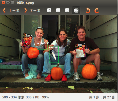
四 用自己的模型在图片上进行目标识别
# -*- coding: utf-8 -*
import numpy as np
import timeit
from PIL import Image
from PIL import ImageDraw
import os
import numpy as np
import matplotlib.pyplot as plt
plt.rcParams['figure.figsize'] = (10, 10)
plt.rcParams['image.interpolation'] = 'nearest'
plt.rcParams['image.cmap'] = 'gray'
# Make sure that the work directory is caffe_root
caffe_root = './'
# modify img_dir to your path of testing images of kitti
#需要测试的集合的图片
img_dir = 'models/knife/test1/'
import os
os.chdir(caffe_root)
import sys
sys.path.insert(0, 'python')
from google.protobuf import text_format
from caffe.proto import caffe_pb2
import caffe
#from _ensemble import *
caffe.set_device(0)
caffe.set_mode_gpu()
#deploy,模型,和labelmap的位置
model_def = 'models/knife/model-v1/SSD_300x300/deploy.prototxt'
model_weights = 'models/knife/model-v1/SSD_300x300/VGG_knife_SSD_300x300_iter_150000.caffemodel'
voc_labelmap_file = caffe_root+'data/VOC_knife/ImageSets/labelmap_knife.prototxt'
#最后标记完保存的路径
save_dir = 'models/knife/result1-150000/'
txt_dir = 'models/knife/result1-150000/'
#f = open (r'out_3d.txt','w')
if not(os.path.exists(txt_dir)):
os.makedirs(txt_dir)
if not(os.path.exists(save_dir)):
os.makedirs(save_dir)
file = open(voc_labelmap_file, 'r')
labelmap = caffe_pb2.LabelMap()
text_format.Merge(str(file.read()), labelmap)
net = caffe.Net(model_def, # defines the structure of the model
model_weights, # contains the trained weights
caffe.TEST) # use test mode (e.g., don't perform dropout)
# input preprocessing: 'data' is the name of the input blob == net.inputs[0]
transformer = caffe.io.Transformer({'data': net.blobs['data'].data.shape})
transformer.set_transpose('data', (2, 0, 1))
transformer.set_mean('data', np.array([104,117,123])) # mean pixel
transformer.set_raw_scale('data', 255) # the reference model operates on images in [0,255] range instead of [0,1]
transformer.set_channel_swap('data', (2,1,0)) # the reference model has channels in BGR order instead of RGB
# set net to batch size of 1
image_width = 300
image_height = 300
net.blobs['data'].reshape(1,3,image_height,image_width)
def get_labelname(labelmap, labels):
num_labels = len(labelmap.item)
labelnames = []
if type(labels) is not list:
labels = [labels]
for label in labels:
found = False
for i in xrange(0, num_labels):
if label == labelmap.item[i].label:
found = True
labelnames.append(labelmap.item[i].display_name)
break
assert found == True
return labelnames
im_names = list(os.walk(img_dir))[0][2]
for im_name in im_names:
img_file = img_dir + im_name
image = caffe.io.load_image(img_file)
transformed_image = transformer.preprocess('data', image)
net.blobs['data'].data[...] = transformed_image
#t1 = timeit.Timer("net.forward()","from __main__ import net")
#print t1.timeit(2)
# Forward pass.
detections = net.forward()['detection_out']
# Parse the outputs.
det_label = detections[0,0,:,1]
det_conf = detections[0,0,:,2]
det_xmin = detections[0,0,:,3]
det_ymin = detections[0,0,:,4]
det_xmax = detections[0,0,:,5]
det_ymax = detections[0,0,:,6]
# Get detections with confidence higher than 0.001
top_indices = [i for i, conf in enumerate(det_conf) if conf >= 0.15]
top_conf = det_conf[top_indices]
top_label_indices = det_label[top_indices].tolist()
top_labels = get_labelname(labelmap, top_label_indices)
top_xmin = det_xmin[top_indices]
top_ymin = det_ymin[top_indices]
top_xmax = det_xmax[top_indices]
top_ymax = det_ymax[top_indices]
#colors = plt.cm.hsv(np.linspace(0, 1, 21)).tolist()
#img = Image.open(img_dir + "%06d.jpg"%(img_idx))
img = Image.open(img_file)
draw = ImageDraw.Draw(img)
for i in xrange(top_conf.shape[0]):
xmin = top_xmin[i] * image.shape[1]
ymin = top_ymin[i] * image.shape[0]
xmax = top_xmax[i] * image.shape[1]
ymax = top_ymax[i] * image.shape[0]
h = float(ymax - ymin)
w = float(xmax - xmin)
#if (w==0) or (h==0):
# continue
#if (h/w >=2)and((xmin<10)or(xmax > 1230)):
# continue
score = top_conf[i]
label_num = top_label_indices[i]
if score > 0.3:
draw.line(((xmin,ymin),(xmin,ymax),(xmax,ymax),(xmax,ymin),(xmin,ymin)),fill=(0,255,0))
draw.text((xmin,ymin),'%s%.2f'%(top_labels[i], score),fill=(255,255,255))
#elif score > 0.02:
# draw.line(((xmin,ymin),(xmin,ymax),(xmax,ymax),(xmax,ymin),(xmin,ymin)),fill=(255,0,255))
# draw.text((xmin,ymin),'%.2f'%(score),fill=(255,255,255))
#img.save(save_dir+"%06d.jpg"%(img_idx))
img.save(save_dir+im_name)然后就会在定义的路径下产生识别好的图片: