自编码器的原理及实现

1. 什么是自编码器

自编码器就是将原始数据进行编码，进行降低维度，发现数据之间的规律的过程。
数据降维比如mnist的图片为28*28像素，将图片向量化之后的得到一个长度为784的向量。在网络训练的过程中，网络只用到该向量之中少量元素，其中的大部分元素对于网络来说是没有用的，自编码器通过无监督学习来提取有用的信息，对于手写数字图片来说可能是颜色为黑色的像素点，将图片中的很大一部分白色像素舍弃，只提取对网络有用的信息，到达降低数据维度的目的。

作用

先对无标注的数据进行自编码器的训练，然后将有标注的数据第一步输入自编码器，自编码器的输出输入到神经网络之中，达到提升网络输出精度的目的。
用于神经网络权重的初始化。

基本形式如下，其中f(x)为编码函数，g(x)为解码函数
$x\overset{f(x)}{\rightarrow}h\overset{g(x)}{\rightarrow}x'$
训练的过程，我们采用下面形式的约束
$x\approx x'$
即设计一个损失函数，让编码器的输入和输出尽可能相似
其中
$x'=g(f(x))$
但自编码器学习的目的不是学习上面这个恒等函数，这可能导致过拟合，我们要自编码器学习的是将稀疏数据到稠密的一个映射，而不是输入和输出完全相等，这样提取的特征才能为后面的网络所用。

损失函数的设计

以mnist数据集为例，设输入x的数据是长度为784的一维向量，编码后h是长度为196的一维向量，解码后x’是长度为784的一维向量。

均方误差（MSE） 用来衡量输入数据和输出数据的相似度。表示如下
$L(x,g(f(x))=E_{x\sim~p_{data}}\left\|x-g(f(x))\right\|^2$
在学习的过程中，均方误差可能变得很小，这样会导过拟合，而我们期望的是一个泛化能力很强的编码器，所以我们加如L1正则化和相对熵(KLD)来抑制过拟合。
L1正则化仅仅作用于编码，因为我们关心的是编码的过程，解码器只是方便显示编码之后的结果。
$\Omega(h)=\lambda\sum\nolimits_{i}\left|h_i\right|$
$h_i$ 是第 $i$ 个神经元的激励值。

相对熵（KL Divergence，KLD）。首先定义隐层神经元j的平均活跃度$ {\hat{\rho}}_j$
$\hat{\rho}_j=\frac{1}{N}\sum\nolimits_{i=1}^{N}{h}^{(i)}_j$
对 $i$ 求和表示对训练集（N个样本）的所有输入取均值，j代表第几个隐层神经元，激励值通常在 $0\sim1$ 之间。对稀疏性的约束就是令神经元的平均活跃度接近稀疏性系数 $\rho:\hat{\rho}_j\approx\rho$ 这个系数通常取接近0的值，从而约束隐层神经元的活跃程度，可以把 $\rho$ 理解成某个神经元被激活的概率。

为了实现这个约束，需要在损失函数中添加一个损失项
$\sum\nolimits_{j=1}^{M}KL(\rho\parallel\hat{\rho}_j)=\sum\nolimits_{j=1}^{M}[\rho\cdot\log\frac{p}{\hat{\rho}_j}+(1-\rho)\cdot\log\frac{1-p}{1-\hat{\rho}_j}]$
KLD是一种衡量两个分布之间差异的方法，式中的 $\rho$ 和 $\hat{\rho}_j$ 分别表示期望和实际的隐层神经元的输出两点分布（两点分别代表饱和和睡眠）的均值和期望。

两种损失函数可定义为下面版本：

L1：
$L(x,g(f(x))=E_{x\sim~p_{data}}\left\|x-g(f(x))\right\|^2+\lambda\sum\nolimits_{i}\left|h_i\right|$
KLD：
$L(x,g(f(x))=E_{x\sim~p_{data}}\left\|x-g(f(x))\right\|^2+\beta\sum_{j=1}^{M}[\rho\cdot\log\frac{p}{\hat{\rho}_j}+(1-\rho)\cdot\log\frac{1-p}{1-\hat{\rho}_j}]$

两种损失函数该如何选择

隐层激活函数类型	重构层激活函数类型	MSE	L1	KLD
Sigmoid	Sigmoid	True	False	True
Relu	Softplus	True	True	False

隐层使用Sigmoid时，隐层输出值在(0,1)之间，可用来计算KLD。隐层使用Relu时，隐层的输出值在 $[0,+\infty)$ ，不能使用KLD。

实现代码如下：

# coding:utf-8

import tensorflow as tf
import tensorlayer as tl
from tensorlayer.layers import *
import numpy as np
import matplotlib.pylab as plt

learning_rate = 0.0001
lambda_l2_w = 0.01
n_epochs = 100
batch_size = 128
print_interval = 200

hidden_size = 196
input_size = 784
image_width = 28
model = 'sigmoid'

X_train, y_train, X_val, y_val, X_test, y_test = tl.files.load_mnist_dataset(path='./data/')

x = tf.placeholder(tf.float32,shape=[None,784],name='x')

print('Build Network')
if model=='relu':
	net = InputLayer(x, name='input')
	net = DenseLayer(net,n_units=hidden_size,act=tf.nn.relu, name='relu1')
	encode_img = net.outputs
	recon_layer1 = DenseLayer(net,n_units=input_size,act=tf.nn.softplus,name='recon_layer1')

if model=='sigmoid':
	net = InputLayer(x, name='input')
	net = DenseLayer(net,n_units=hidden_size,act=tf.nn.sigmoid, name='sigmoid1')
	encode_img = net.outputs
	recon_layer1 = DenseLayer(net,n_units=input_size,act=tf.nn.sigmoid,name='recon_layer1')

y = recon_layer1.outputs
train_params = recon_layer1.all_params[-4:]

mse = tf.reduce_sum(tf.squared_difference(y,x),1)
mse = tf.reduce_mean(mse)

# w1 和 w2 采用L2正则化
L2_w = tf.contrib.layers.l2_regularizer(lambda_l2_w)(train_params[0])+\
       tf.contrib.layers.l2_regularizer(lambda_l2_w)(train_params[2])

# 稀疏性约束
activation_out = recon_layer1.all_layers[-2]
L1_a = 0.001 * tf.reduce_mean(activation_out)

# 相对熵（KLD）
beta = 0.5
rho = 0.15
p_hat = tf.reduce_mean(activation_out,0)
KLD = beta * tf.reduce_sum(rho * tf.log(tf.divide(rho,p_hat)) +
                            (1-rho) * tf.log((1-rho)/(tf.subtract(float(1),p_hat))))

# 联合损失函数
if model=='sigmoid':
	cost = mse + L2_w + KLD
if model=='relu':
	cost = mse + L2_w + L1_a

# 定义优化器
train_op = tf.train.AdamOptimizer(learning_rate).minimize(cost)
saver = tf.train.Saver()

# 模型训练
total_batch = X_train.shape[0] // batch_size

with tf.Session() as sess:
	sess.run(tf.global_variables_initializer())

	for epoch in range(n_epochs):
		avg_cost = 0
		for i in range(total_batch):
			batch_x,batch_y =X_train[i*batch_size:(i+1)*batch_size],y_train[i*batch_size:(i+1)*batch_size]
			batch_x = np.array(batch_x).astype(np.float32)
			batch_cost, _ = sess.run([cost, train_op], feed_dict={x: batch_x})
			if not i % print_interval:
				print('Minibatch: %03d | Cost:  %.3f' % (i + 1, batch_cost))
		print('Epoch:   %03d | AvgCost:  %.3f' % (epoch + 1, avg_cost / i + 1))
	saver.save(sess,save_path='./model/3-101.ckpt')

# 恢复参数
n_images=15
fig,axes=plt.subplots(nrows=2,ncols=n_images,sharex=True,sharey=True,figsize=(20,2.5))

test_images = X_test[:n_images]

with tf.Session() as sess:
	# 加载训练好的模型
	saver.restore(sess,save_path='./model/3-101.ckpt')

	# 获取重构参数
	decoded = sess.run(recon_layer1.outputs,feed_dict={x:test_images})
	# 恢复编码器的权重参数
	if model=='relu':
		weights = sess.run(tl.layers.get_variables_with_name('relu1/W:0',False,True))
	if model=='sigmoid':
		weights = sess.run(tl.layers.get_variables_with_name('sigmoid1/W:0',False,True))

	# 获取解码器的权重参数
	recon_weights = sess.run(tl.layers.get_variables_with_name('recon_layer1/W:0',False,True))
	recon_bias = sess.run(tl.layers.get_variables_with_name('recon_layer1/b:0',False,True))
	for i in range(n_images):
		for ax,img in zip(axes,[test_images,decoded]):
			ax[i].imshow(img[i].reshape(image_width,image_width),cmap='binary')
	plt.show()

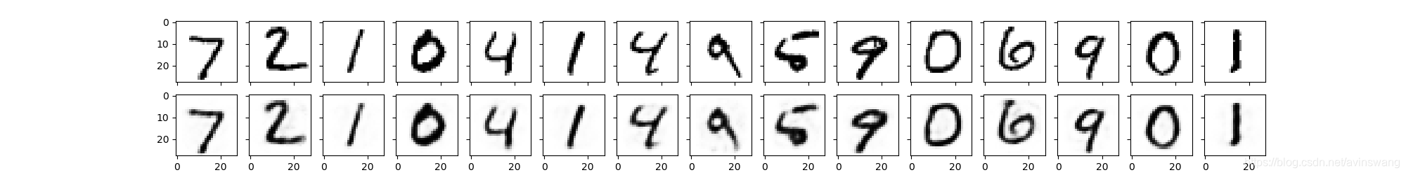
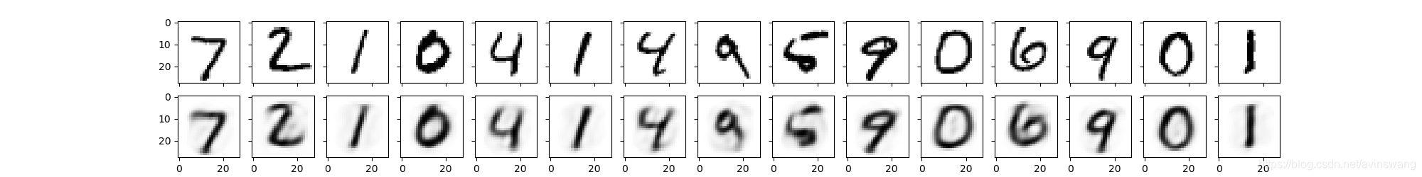
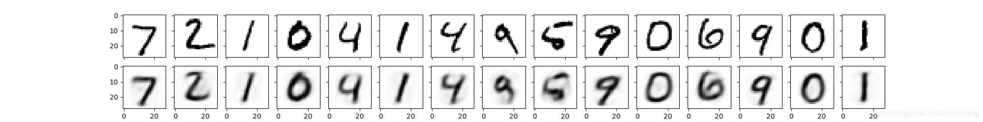
实验结果:

MSE

在这里插入图片描述

MSE+L2

在这里插入图片描述

MSE+L2+KLD

在这里插入图片描述

总结：

自编码器通过监督学习来发现数据集内部特征，提取有用信息，达到降维的目的。在现实中存在大量无标注的数据，先用这部分数据训练一个自编码器，在神经网络训练过程中，先将数据喂入自编码器，自编码器输出的结果再喂入神经网络进行训练。通过这种操作达到提升训练效果的目的。

这个自编码器不是说输出数据和输入数据的相似度越高越好，相似度太高可能出现过拟合的情况，我们所希望的是自编码器对同一类型的数据都具有编码能力，即要求自编码器有很强的泛化能力。为了达到这个目的，在实验中对编码器增加正则化和KLD惩罚项，使得自编码器学习到稀疏性特征。需要注意的是两个版本的损失函数的使用场景各不相同。

注

参考《一起玩转TensorLayer》