第二章：单变量线性回归

单变量线性回归（Univariate linear regression）

介绍

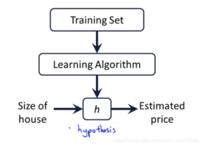
一个数据集也被称为一个训练集

• 数据集的表示
  m ：数据集样本容量
  (x,y) ：一个样本，x为输入，y为输出
  $x^{(i)}$ ：第i个样本的输入 ， $y^{(i)}$：第i个样本的输出
• 学习算法的任务就是根据训练集来输出一个函数，这个函数能够根据input来预测output
  
  定义代价函数（平方误差代价函数：square error cost function ）
  $J(\theta_0,\theta_1)=\frac{1}{2m}\sum_i^n(h_\theta(x^{(i)})-y^{(i)})^2$
  其中 $h_\theta(x^{i})=\theta_0+\theta_1x^{(i)}$
  为我们要求出的预测函数。
  我们要做的事是求出 $\theta_0和\theta_1$使得代价函数最小。
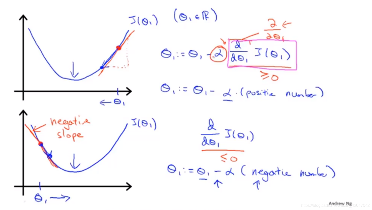
• ** 梯度下降法**（ Gradient Descent）
  给出一个函数 $J(\theta_0,\theta_1,...,\theta_n)$梯度下降法可以求得其取最小值时，参数 $\theta_0,\theta_1,...\theta_n$的值。
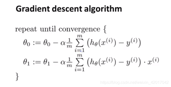
  • 过程（此处的梯度下降法为“Batch” Gradient Descent，每一步更新都会遍历整个数据集，还有其他的梯度下降法）
    repeat until convergence {
    $\theta_j := \theta_j-\alpha\frac{\partial}{\partial \theta_j}J(\theta_0,\theta_1)$ $(j=0\ and\ j=1)$
    }
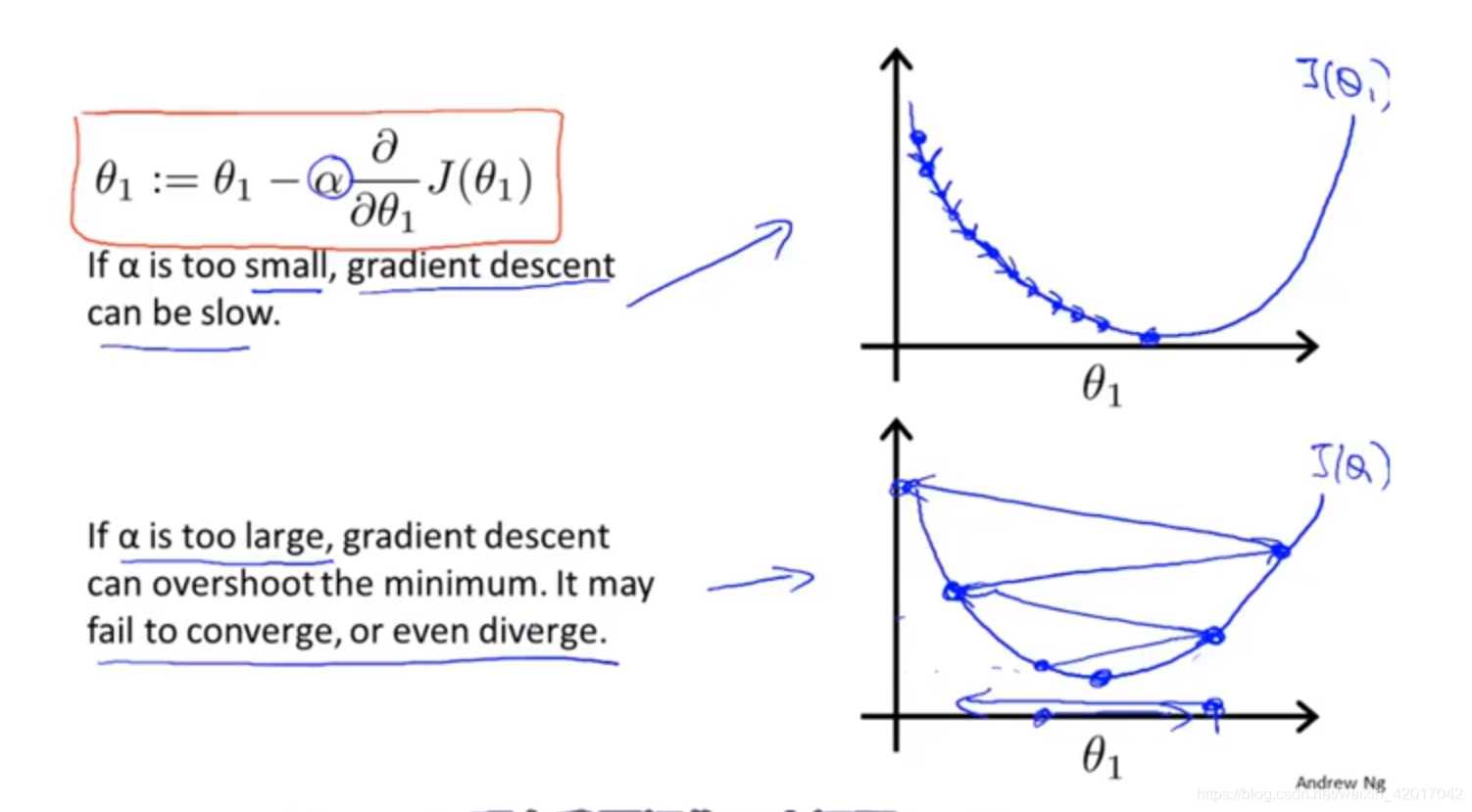
    $\alpha$被称为学习率（learning rate），它决定了梯度下降的速度
  • 同时更新
    $temp0 := \theta_0-\frac{\partial}{\partial \theta_0}J(\theta_0,\theta_1)$
    $temp1 := \theta_1-\frac{\partial}{\partial \theta_1}J(\theta_0,\theta_1)$
    $\theta_0:=temp0$
    $\theta_1:=temp1$
  • 梯度下降法单变量时的直观解释
    
  • 学习率 $\alpha$的直观解释
    

线性回归的梯度下降

根据公式，求偏导代入即可