YOLO模型介绍
简介
YOLO为一种新的目标检测方法,该方法的特点是实现快速检测的同时还达到较高的准确率。作者将目标检测任务看作目标区域预测和类别预测的回归问题。该方法采用单个神经网络直接预测物品边界和类别概率,实现端到端的物品检测。同时,该方法检测速非常快,基础版可以达到45帧/s的实时检测;FastYOLO可以达到155帧/s。与当前最好系统相比,YOLO目标区域定位误差更大,但是背景预测的假阳性优于当前最好的方法。 基于深度学习方法的一个特点就是实现端到端的检测。相对于其它目标检测与识别方法(比如Fast R-CNN)将目标识别任务分类目标区域预测和类别预测等多个流程,YOLO将目标区域预测和目标类别预测整合于单个神经网络模型中,实现在准确率较高的情况下快速目标检测与识别,更加适合现场应用环境。后续研究,可以进一步优化YOLO网络结构,提高YOLO准确率。YOLO类型的端到端的实时目标检测方法是一个很好的研究方向。
2.1 网络结构
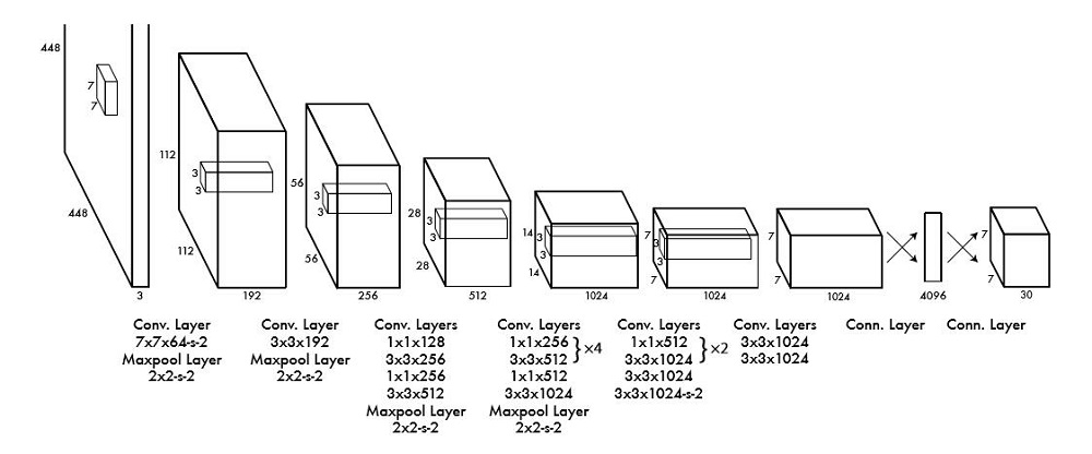
模型采用卷积神经网络结构。开始的卷积层提取图像特征,全连接层预测输出概率。模型结构类似于GoogleNet,如图3所示。作者还训练了YOLO的快速版本(fast YOLO)。Fast YOLO模型卷积层和filter更少。最终输出为7×7×30的tensor。
核心思想
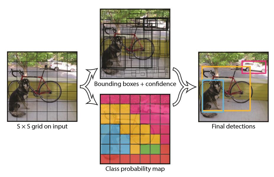
YOLO的工作过程分为以下几个过程:(1) 将原图划分为SxS的网格。如果一个目标的中心落入某个格子,这个格子就负责检测该目标。(2) 每个网格要预测B个bounding boxes,以及C个类别概率Pr(classi|object)。这里解释一下,C是网络分类总数,由训练时决定。在作者给出的demo中C=20,包含以下类别: 人person鸟bird、猫cat、牛cow、狗dog、马horse、羊sheep飞机aeroplane、自行车bicycle、船boat、巴士bus、汽车car、摩托车motorbike、火车train瓶子bottle、椅子chair、餐桌dining table、盆景potted plant、沙发sofa、显示器tv/monitor在YOLO中,每个格子只有一个C类别,即相当于忽略了B个bounding boxes,每个格子只判断一次类别,这样做非常简单粗暴。(3) 每个bounding box除了要回归自身的位置之外,还要附带预测一个confidence值。这个confidence代表了所预测的box中含有目标的置信度和这个bounding box预测的有多准两重信息:
如果有目标落中心在格子里Pr(Object)=1;否则Pr(Object)=0。 第二项是预测的bounding box和实际的ground truth之间的IOU。 缩进所以,每个bounding box都包含了5个预测量:(x, y, w, h, confidence),其中(x, y)代表预测box相对于格子的中心,(w, h)为预测box相对于图片的width和height比例,confidence就是上述置信度。需要说明,这里的x, y, w和h都是经过归一化的,之后有解释。(4) 由于输入图像被分为SxS网格,每个网格包括5个预测量:(x, y, w, h, confidence)和一个C类,所以网络输出是SxSx(5xB+C)大小(5) 在检测目标的时候,每个网格预测的类别条件概率和bounding box预测的confidence信息相乘,就得到每个bounding box的class-specific confidence score:
显然这个class-specific confidence score既包含了bounding box最终属于哪个类别的概率,又包含了bounding box位置的准确度。最后设置一个阈值与class-specific confidence score对比,过滤掉score低于阈值的boxes,然后对score高于阈值的boxes进行非极大值抑制(NMS, non-maximum suppression)后得到最终的检测框体。
3. YOLO中的Bounding Box Normalization缩进YOLO在实现中有一个重要细节,即对bounding box的坐标(x, y, w, h)进行了normalization,以便进行回归。作者认为这是一个非常重要的细节。在原文2.2 Traing节中有如下一段:Our final layer predicts both class probabilities and bounding box coordinates. We normalize the bounding box width and height by the image width and height so that they fall between 0 and 1. We parametrize the bounding box x and y coordinates to be offsets of a particular grid cell location so they are also bounded between 0 and 1.缩进接下来分析一下到底如何实现。


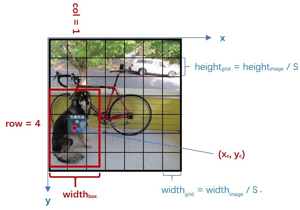
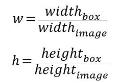
如图4,在YOLO中输入图像被分为SxS网格。假设有一个bounding box(如图4红框),其中心刚好落在了(row,col)网格中,则这个网格需要负责预测整个红框中的dog目标。假设图像的宽为widthimage,高为heightimage;红框中心在(xc,yc),宽为widthbox,高为heightbox那么:(1) 对于bounding box的宽和高做如下normalization,使得输出宽高介于0~1:
(2) 使用(row, col)网格的offset归一化bounding box的中心坐标:
经过上述公式得到的normalization的(x, y, w, h),再加之前提到的confidence,共同组成了一个真正在网络中用于回归的bounding box; 而当网络在Test阶段(x,y,w,h)经过反向解码又可得到目标在图像坐标系的框,相关解码代码在darknet框架detection_layer.c中的get_detection_boxes()函数,关键部分如下:

boxes[index].x = (predictions[box_index + 0] + col) / l.side * w;
boxes[index].y = (predictions[box_index + 1] + row) / l.side * h;
boxes[index].w = pow(predictions[box_index + 2], (l.sqrt?2:1)) * w;
boxes[index].h = pow(predictions[box_index + 3], (l.sqrt?2:1)) * h;
YOLO代价函数
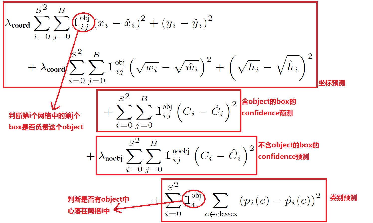
缩进对于任何一种网络,loss都是非常重要的,直接决定网络效果的好坏。YOLO的Loss函数设计时主要考虑了以下3个方面(1) bounding box的(x, y, w, h)的坐标预测误差。 缩进在检测算法的实际使用中,一般都有这种经验:对不同大小的bounding box预测中,相比于大box大小预测偏一点,小box大小测偏一点肯定更不能被忍受。所以在Loss中同等对待大小不同的box是不合理的。为了解决这个问题,作者用了一个比较取巧的办法,即对w和h求平方根进行回归。从后续效果来看,这样做很有效,但是也没有完全解决问题。(2) bounding box的confidence预测误差 缩进由于绝大部分网格中不包含目标,导致绝大部分box的confidence=0,所以在设计confidence误差时同等对待包含目标和不包含目标的box也是不合理的,否则会导致模型不稳定。作者在不含object的box的confidence预测误差中乘以惩罚权重λnoobj=0.5。 缩进除此之外,同等对待4个值(x, y, w, h)的坐标预测误差与1个值的conference预测误差也不合理,所以作者在坐标预测误差误差之前乘以权重λcoord=5(至于为什么是5而不是4,我也不知道T_T)。(3) 分类预测误差 缩进即每个box属于什么类别,需要注意一个网格只预测一次类别,即默认每个网格中的所有B个bounding box都是同一类。所以,YOLO的最终误差为下:Loss = λcoord * 坐标预测误差 + (含object的box confidence预测误差 + λnoobj * 不含object的box confidence预测误差) + 类别预测误差
网络实现
标签定义
标签是训练时必不可少的数据,理解标签怎么定义也是理解YOLO训练过程的第一步,下面就描述下标签定义的过程。
- 读取图片对于的 image.xml文件,文件里面记录了一张图片所包含物体的类型,以及对应的位置。解析出.xml里面的物体以及对应位置。
- 将图片分成 7 * 7的大小,称作box_cenn,然后计算出每个物体的中心落在哪个区域 cell里面。
- 将有物体的cell标记为1,表示该cell 含有物体,并记录其boxes的具体信息(xc, yc, w, h)
- 然后再标出这个物体的类别,one-hot形式,假如有三个类别,该类别为最后一个类别,则表示为[0, 0, 1]
所以对于YOLO 20个类别的识别中,如果每个cell只用于预测一个类别,则 一个图片的 Label shape为 [1, 25]
备注:(如果想一个cell预测多个类别,需要使用anchor机制,可自行了解)def load_pascal_annotation(self, index):
"""
Load image and bounding boxes info from XML file in the PASCAL VOC
format.
"""
imname = os.path.join(self.data_path, 'JPEGImages', index + '.jpg')
im = cv2.imread(imname)
h_ratio = 1.0 * self.image_size / im.shape[0]
w_ratio = 1.0 * self.image_size / im.shape[1]
# im = cv2.resize(im, [self.image_size, self.image_size])
label = np.zeros((self.cell_size, self.cell_size, 25))
filename = os.path.join(self.data_path, 'Annotations', index + '.xml')
tree = ET.parse(filename)
objs = tree.findall('object')
for obj in objs:
bbox = obj.find('bndbox')
# Make pixel indexes 0-based
x1 = max(min((float(bbox.find('xmin').text) - 1) * w_ratio, self.image_size - 1), 0)
y1 = max(min((float(bbox.find('ymin').text) - 1) * h_ratio, self.image_size - 1), 0)
x2 = max(min((float(bbox.find('xmax').text) - 1) * w_ratio, self.image_size - 1), 0)
y2 = max(min((float(bbox.find('ymax').text) - 1) * h_ratio, self.image_size - 1), 0)
cls_ind = self.class_to_ind[obj.find('name').text.lower().strip()]
boxes = [(x2 + x1) / 2.0, (y2 + y1) / 2.0, x2 - x1, y2 - y1]
x_ind = int(boxes[0] * self.cell_size / self.image_size)
y_ind = int(boxes[1] * self.cell_size / self.image_size)
if label[y_ind, x_ind, 0] == 1:
continue
label[y_ind, x_ind, 0] = 1
label[y_ind, x_ind, 1:5] = boxes
label[y_ind, x_ind, 5 + cls_ind] = 1
return label, len(objs)
网络定义
YOLO 网络是端到端的网络,相对于其他的目标检测模型,该模型要简单很多。
def build_network(self,
                      images,
                      num_outputs,
                      alpha,
                      keep_prob=0.5,
                      is_training=True,
                      scope='yolo'):
        with tf.variable_scope(scope):
            with slim.arg_scope([slim.conv2d, slim.fully_connected],
                                activation_fn=leaky_relu(alpha),
                                weights_initializer=tf.truncated_normal_initializer(0.0, 0.01),
                                weights_regularizer=slim.l2_regularizer(0.0005)):
                net = tf.pad(images, np.array([[0, 0], [3, 3], [3, 3], [0, 0]]), name='pad_1')
                net = slim.conv2d(net, 64, 7, 2, padding='VALID', scope='conv_2')
                net = slim.max_pool2d(net, 2, padding='SAME', scope='pool_3')
                net = slim.conv2d(net, 192, 3, scope='conv_4')
                net = slim.max_pool2d(net, 2, padding='SAME', scope='pool_5')
                net = slim.conv2d(net, 128, 1, scope='conv_6')
                net = slim.conv2d(net, 256, 3, scope='conv_7')
                net = slim.conv2d(net, 256, 1, scope='conv_8')
                net = slim.conv2d(net, 512, 3, scope='conv_9')
                net = slim.max_pool2d(net, 2, padding='SAME', scope='pool_10')
                net = slim.conv2d(net, 256, 1, scope='conv_11')
                net = slim.conv2d(net, 512, 3, scope='conv_12')
                net = slim.conv2d(net, 256, 1, scope='conv_13')
                net = slim.conv2d(net, 512, 3, scope='conv_14')
                net = slim.conv2d(net, 256, 1, scope='conv_15')
                net = slim.conv2d(net, 512, 3, scope='conv_16')
                net = slim.conv2d(net, 256, 1, scope='conv_17')
                net = slim.conv2d(net, 512, 3, scope='conv_18')
                net = slim.conv2d(net, 512, 1, scope='conv_19')
                net = slim.conv2d(net, 1024, 3, scope='conv_20')
                net = slim.max_pool2d(net, 2, padding='SAME', scope='pool_21')
                net = slim.conv2d(net, 512, 1, scope='conv_22')
                net = slim.conv2d(net, 1024, 3, scope='conv_23')
                net = slim.conv2d(net, 512, 1, scope='conv_24')
                net = slim.conv2d(net, 1024, 3, scope='conv_25')
                net = slim.conv2d(net, 1024, 3, scope='conv_26')
                net = tf.pad(net, np.array([[0, 0], [1, 1], [1, 1], [0, 0]]), name='pad_27')
                net = slim.conv2d(net, 1024, 3, 2, padding='VALID', scope='conv_28')
                net = slim.conv2d(net, 1024, 3, scope='conv_29')
                net = slim.conv2d(net, 1024, 3, scope='conv_30')
                net = tf.transpose(net, [0, 3, 1, 2], name='trans_31')
                net = slim.flatten(net, scope='flat_32')
                net = slim.fully_connected(net, 512, scope='fc_33')
                net = slim.fully_connected(net, 4096, scope='fc_34')
                net = slim.dropout(net, keep_prob=keep_prob,
                                   is_training=is_training, scope='dropout_35')
                net = slim.fully_connected(net, num_outputs,
                                           activation_fn=None, scope='fc_36')
        return net
网络训练
网络模型很简单,难点就在于怎么定义我们的 代价函数(cost function),根据上图的代价公式这里直接上代码,注释写在代码里面 了。
def loss_layer(self, predicts, labels, scope='loss_layer'):
        with tf.variable_scope(scope):
            #预测结果是 batch_zise*7*7*30的矩阵,首先将预测结果分开,每个cell是否含有物体[predict_classes]、类别概率[predict_scales]、boudingbox信息[predict_boxes]
            predict_classes = tf.reshape(predicts[:, :self.boundary1], [self.batch_size, self.cell_size, self.cell_size, self.num_class])
            predict_scales = tf.reshape(predicts[:, self.boundary1:self.boundary2], [self.batch_size, self.cell_size, self.cell_size, self.boxes_per_cell])
            predict_boxes = tf.reshape(predicts[:, self.boundary2:], [self.batch_size, self.cell_size, self.cell_size, self.boxes_per_cell, 4])
            #同样把我们之前定义好的label取出,按照预测的形式 分成三个部分,这里注意,预测时每个cell预测结果有30个,分别是2个位置信息boxes(8个值),2个位置信息的置信度(2个值),20个类别概率(20个值),一起刚好30个值。【备注:YOLO 预测时每个cell会预测一个类别,对于这一个类别会预测两个位置信息,最后预测会根据这个两个位置信息的置信度来选择置信度最大的boundingbox(预测时中间还包括置信度与概率乘积是否大于某个阈值,对于预测出的box做非极大值抑制)】
            response = tf.reshape(labels[:, :, :, 0], [self.batch_size, self.cell_size, self.cell_size, 1])
            boxes = tf.reshape(labels[:, :, :, 1:5], [self.batch_size, self.cell_size, self.cell_size, 1, 4])
            #因为样本只定义了一个boxes,所以这里统一增加一个一样的置信度和boundingbox 变成 25+1+4 = 30
            boxes = tf.tile(boxes, [1, 1, 1, self.boxes_per_cell, 1]) / self.image_size
            classes = labels[:, :, :, 5:]
            #预测结果是经过归一化的,每个 x,y代表的是对于 一个cell的偏置,这里进行转换[xc,yc,sqrt(w),sqrt(h)] -> [x,y,w,h]  主要目的是进行IOU计算
            offset = tf.constant(self.offset, dtype=tf.float32)
            offset = tf.reshape(offset, [1, self.cell_size, self.cell_size, self.boxes_per_cell])
            offset = tf.tile(offset, [self.batch_size, 1, 1, 1])
            predict_boxes_tran = tf.stack([(predict_boxes[:, :, :, :, 0] + offset) / self.cell_size,
                                           (predict_boxes[:, :, :, :, 1] + tf.transpose(offset, (0, 2, 1, 3))) / self.cell_size,
                                           tf.square(predict_boxes[:, :, :, :, 2]),
                                           tf.square(predict_boxes[:, :, :, :, 3])])
            predict_boxes_tran = tf.transpose(predict_boxes_tran, [1, 2, 3, 4, 0])
            #iou 代表了我们预测的box与真实box的交并比,可以理解为当前boxes的置信度,根据这个值来调节预测的置信度的值
            iou_predict_truth = self.calc_iou(predict_boxes_tran, boxes)

            # calculate I tensor [BATCH_SIZE, CELL_SIZE, CELL_SIZE, BOXES_PER_CELL]
            object_mask = tf.reduce_max(iou_predict_truth, 3, keep_dims=True)
            object_mask = tf.cast((iou_predict_truth >= object_mask), tf.float32) * response

            # calculate no_I tensor [CELL_SIZE, CELL_SIZE, BOXES_PER_CELL]
            noobject_mask = tf.ones_like(object_mask, dtype=tf.float32) - object_mask
            #这里同样将我们的标签进行归一化 [x,y ,w, h] ->[xc, yc, sqrt(w), sqrt(h)]
            boxes_tran = tf.stack([boxes[:, :, :, :, 0] * self.cell_size - offset,
                                   boxes[:, :, :, :, 1] * self.cell_size - tf.transpose(offset, (0, 2, 1, 3)),
                                   tf.sqrt(boxes[:, :, :, :, 2]),
                                   tf.sqrt(boxes[:, :, :, :, 3])])
            boxes_tran = tf.transpose(boxes_tran, [1, 2, 3, 4, 0])

            #根据上图的loss公式进行loss函数的计算
            # class_loss  response代表标签实际有物体的cell
            class_delta = response * (predict_classes - classes)
            class_loss = tf.reduce_mean(tf.reduce_sum(tf.square(class_delta), axis=[1, 2, 3]), name='class_loss') * self.class_scale

            # object_loss       object_mask 代表预测有物体,且标签实际也有物体的 cell
            object_delta = object_mask * (predict_scales - iou_predict_truth)
            object_loss = tf.reduce_mean(tf.reduce_sum(tf.square(object_delta), axis=[1, 2, 3]), name='object_loss') * self.object_scale

            # noobject_loss
            noobject_delta = noobject_mask * predict_scales
            noobject_loss = tf.reduce_mean(tf.reduce_sum(tf.square(noobject_delta), axis=[1, 2, 3]), name='noobject_loss') * self.noobject_scale

            # coord_loss
            coord_mask = tf.expand_dims(object_mask, 4)
            boxes_delta = coord_mask * (predict_boxes - boxes_tran)
            coord_loss = tf.reduce_mean(tf.reduce_sum(tf.square(boxes_delta), axis=[1, 2, 3, 4]), name='coord_loss') * self.coord_scale

            tf.losses.add_loss(class_loss)
            tf.losses.add_loss(object_loss)
            tf.losses.add_loss(noobject_loss)
            tf.losses.add_loss(coord_loss)

#IOU计算
def calc_iou(self, boxes1, boxes2, scope='iou'):
        """calculate ious
        Args:
          boxes1: 4-D tensor [CELL_SIZE, CELL_SIZE, BOXES_PER_CELL, 4]  ====> (x_center, y_center, w, h)
          boxes2: 1-D tensor [CELL_SIZE, CELL_SIZE, BOXES_PER_CELL, 4] ===> (x_center, y_center, w, h)
        Return:
          iou: 3-D tensor [CELL_SIZE, CELL_SIZE, BOXES_PER_CELL]
        """
        with tf.variable_scope(scope):
            boxes1 = tf.stack([boxes1[:, :, :, :, 0] - boxes1[:, :, :, :, 2] / 2.0,
                               boxes1[:, :, :, :, 1] - boxes1[:, :, :, :, 3] / 2.0,
                               boxes1[:, :, :, :, 0] + boxes1[:, :, :, :, 2] / 2.0,
                               boxes1[:, :, :, :, 1] + boxes1[:, :, :, :, 3] / 2.0])
            boxes1 = tf.transpose(boxes1, [1, 2, 3, 4, 0])

            boxes2 = tf.stack([boxes2[:, :, :, :, 0] - boxes2[:, :, :, :, 2] / 2.0,
                               boxes2[:, :, :, :, 1] - boxes2[:, :, :, :, 3] / 2.0,
                               boxes2[:, :, :, :, 0] + boxes2[:, :, :, :, 2] / 2.0,
                               boxes2[:, :, :, :, 1] + boxes2[:, :, :, :, 3] / 2.0])
            boxes2 = tf.transpose(boxes2, [1, 2, 3, 4, 0])

            # calculate the left up point & right down point
            lu = tf.maximum(boxes1[:, :, :, :, :2], boxes2[:, :, :, :, :2])
            rd = tf.minimum(boxes1[:, :, :, :, 2:], boxes2[:, :, :, :, 2:])

            # intersection
            intersection = tf.maximum(0.0, rd - lu)
            inter_square = intersection[:, :, :, :, 0] * intersection[:, :, :, :, 1]

            # calculate the boxs1 square and boxs2 square
            square1 = (boxes1[:, :, :, :, 2] - boxes1[:, :, :, :, 0]) * \
                (boxes1[:, :, :, :, 3] - boxes1[:, :, :, :, 1])
            square2 = (boxes2[:, :, :, :, 2] - boxes2[:, :, :, :, 0]) * \
                (boxes2[:, :, :, :, 3] - boxes2[:, :, :, :, 1])

            union_square = tf.maximum(square1 + square2 - inter_square, 1e-10)

        return tf.clip_by_value(inter_square / union_square, 0.0, 1.0)
网络预测
def interpret_output(self, output):
        probs = np.zeros((self.cell_size, self.cell_size,
                          self.boxes_per_cell, self.num_class))
        #将预测结果分开,1.类别概率20个  2.置信度2个 3.boxes 8个
        class_probs = np.reshape(output[0:self.boundary1], (self.cell_size, self.cell_size, self.num_class))
        scales = np.reshape(output[self.boundary1:self.boundary2], (self.cell_size, self.cell_size, self.boxes_per_cell))
        boxes = np.reshape(output[self.boundary2:], (self.cell_size, self.cell_size, self.boxes_per_cell, 4))
        offset = np.transpose(np.reshape(np.array([np.arange(self.cell_size)] * self.cell_size * self.boxes_per_cell),
                                         [self.boxes_per_cell, self.cell_size, self.cell_size]), (1, 2, 0))
        #把已经归一化后的 x,y,w,h   变回原来的值。
          boxes[:, :, :, 0] += offset
        boxes[:, :, :, 1] += np.transpose(offset, (1, 0, 2))
        boxes[:, :, :, :2] = 1.0 * boxes[:, :, :, 0:2] / self.cell_size
        boxes[:, :, :, 2:] = np.square(boxes[:, :, :, 2:])

        boxes *= self.image_size
        #计算 置信度与类别概率的乘积
        for i in range(self.boxes_per_cell):
            for j in range(self.num_class):
                probs[:, :, i, j] = np.multiply(
                    class_probs[:, :, j], scales[:, :, i])
        #将乘积小于threshold的值过滤掉
        filter_mat_probs = np.array(probs >= self.threshold, dtype='bool')

        filter_mat_boxes = np.nonzero(filter_mat_probs)
        boxes_filtered = boxes[filter_mat_boxes[0],
                               filter_mat_boxes[1], filter_mat_boxes[2]]
        probs_filtered = probs[filter_mat_probs]
        #对于没有过滤掉的值,找到每个cell的置信度与类别概率的最大乘积
        classes_num_filtered = np.argmax(filter_mat_probs, axis=3)[filter_mat_boxes[
            0], filter_mat_boxes[1], filter_mat_boxes[2]]
        #排序 然后使用于 MNS 再次过滤
        argsort = np.array(np.argsort(probs_filtered))[::-1]
        boxes_filtered = boxes_filtered[argsort]
        probs_filtered = probs_filtered[argsort]
        classes_num_filtered = classes_num_filtered[argsort]

        for i in range(len(boxes_filtered)):
            if probs_filtered[i] == 0:
                continue
            for j in range(i + 1, len(boxes_filtered)):
                if self.iou(boxes_filtered[i], boxes_filtered[j]) > self.iou_threshold:
                    probs_filtered[j] = 0.0

        filter_iou = np.array(probs_filtered > 0.0, dtype='bool')
        boxes_filtered = boxes_filtered[filter_iou]
        probs_filtered = probs_filtered[filter_iou]
        classes_num_filtered = classes_num_filtered[filter_iou]
        #得到预测结果
        result = []
        for i in range(len(boxes_filtered)):
            result.append([self.classes[classes_num_filtered[i]], boxes_filtered[i][0], boxes_filtered[
                          i][1], boxes_filtered[i][2], boxes_filtered[i][3], probs_filtered[i]])

        return result