第2章 感知机(Perceptron)代码实现

上一篇：【第1章课后习题参考解答】 ========================================================================= 【回到目录】 ========================================================================= 下一篇：【[第2章课后习题参考解答]】

import pandas as pd
import numpy as np
from sklearn.datasets import load_iris
import matplotlib.pyplot as plt
#
# load data
iris = load_iris()
#这里不借助DataFrame也可以，直接把X, y = iris.data, iris.target
df = pd.DataFrame(iris.data, columns=iris.feature_names)
df['label'] = iris.target
# print(df.columns)
#'sepal length (cm)', 'sepal width (cm)', 'petal length (cm)','petal width (cm)', 'label' 原来的列名
df.columns = ['sepal length', 'sepal width', 'petal length', 'petal width', 'label']

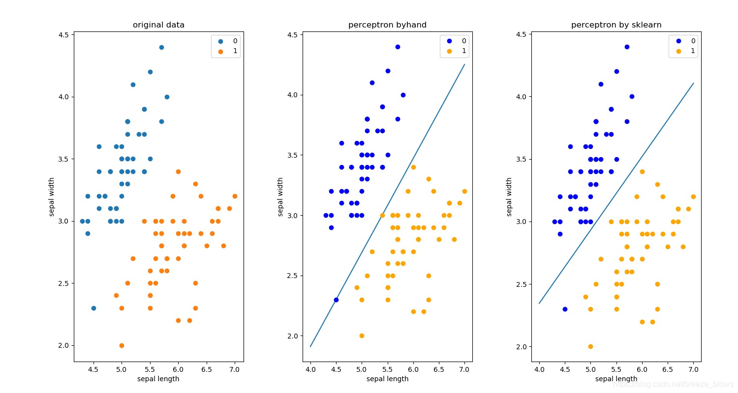
plt.figure(figsize=(15, 8))
plt.subplot(131)
plt.scatter(df[:50]['sepal length'], df[:50]['sepal width'], label='0')
plt.scatter(df[50:100]['sepal length'], df[50:100]['sepal width'], label='1')
plt.xlabel('sepal length')
plt.ylabel('sepal width')
plt.title('original data')
plt.legend()




data = np.array(df.iloc[:100, [0, 1, -1]]) #这里不能用df[:100][0, 1, -1]
X, y = data[:,:-1], data[:,-1]
y = np.array([1 if i == 1 else -1 for i in y])

# 数据线性可分，二分类数据
# 此处为一元一次线性方程

class Model:
    def __init__(self):
        self.w = np.ones(len(data[0]) - 1, dtype=np.float32)
        self.b = 0
        self.l_rate = 0.1
        # self.data = data

    def sign(self, x, w, b):
        y = np.dot(x, w) + b
        return y


    # 随机梯度下降法
    def fit(self, X_train, y_train):
        is_wrong = False
        while not is_wrong:
            wrong_count = 0
            for d in range(len(X_train)):
                X = X_train[d]
                y = y_train[d]
                if y * self.sign(X, self.w, self.b) <= 0:
                    self.w = self.w + self.l_rate * np.dot(y, X)
                    self.b = self.b + self.l_rate * y
                    wrong_count += 1
            if wrong_count == 0:
                is_wrong = True
        return 'Perceptron Model!'




perceptron = Model()
perceptron.fit(X, y)

x_points = np.linspace(4, 7, 10)
y_ = -(perceptron.w[0]*x_points + perceptron.b)/perceptron.w[1]
plt.subplot(132)
plt.plot(x_points, y_)
plt.plot(data[:50, 0], data[:50, 1], 'bo', color='blue', label='0') #用scatter也可以
plt.plot(data[50:100, 0], data[50:100, 1], 'bo', color='orange', label='1')
plt.xlabel('sepal length')
plt.ylabel('sepal width')
plt.title('perceptron byhand')
plt.legend()


from sklearn.linear_model import Perceptron

clf = Perceptron(fit_intercept=False, max_iter=1000, shuffle=False) #fit_intercept表示是否保留截距
clf.fit(X, y)

# Weights assigned to the features.
print(clf.coef_) #二维array

# 截距 Constants in decision function.
print(clf.intercept_)
x_ponits = np.arange(4, 8)
y_ = -(clf.coef_[0][0]*x_ponits + clf.intercept_)/clf.coef_[0][1]
plt.subplot(133)
plt.plot(x_ponits, y_)

plt.plot(data[:50, 0], data[:50, 1], 'bo', color='blue', label='0')
plt.plot(data[50:100, 0], data[50:100, 1], 'bo', color='orange', label='1')
plt.xlabel('sepal length')
plt.ylabel('sepal width')
plt.title('perceptron by sklearn')
plt.legend()

plt.subplots_adjust(top=0.92, bottom=0.08, left=0.10, right=0.95, hspace=0.25,
                        wspace=0.35) #调整子图间距
plt.savefig("demo.jpg")
plt.show()