第1章 统计学习方法概论(LeastSquaresMethod)代码实现

上一篇：【目录】====== 【回到目录】====== 下一篇：【第一章课后习题参考解答】

import numpy as np
from scipy.optimize import leastsq
import matplotlib.pyplot as plt

# 目标函数
def real_func(x):
    return np.sin(2*np.pi*x)

# 多项式
def fit_func(p, x):
    f = np.poly1d(p)
    return f(x)

# 残差
def residuals_func(p, x, y):
    ret = fit_func(p, x) - y #注意此处没有平方
    return ret

regularization = 0.0001

#正则化之后的残差
def residuals_func_regularization(p, x, y):
    ret = fit_func(p, x) - y
    ret = np.append(ret, np.sqrt(0.5*regularization*np.square(p))) # L2范数作为正则化项
    return ret


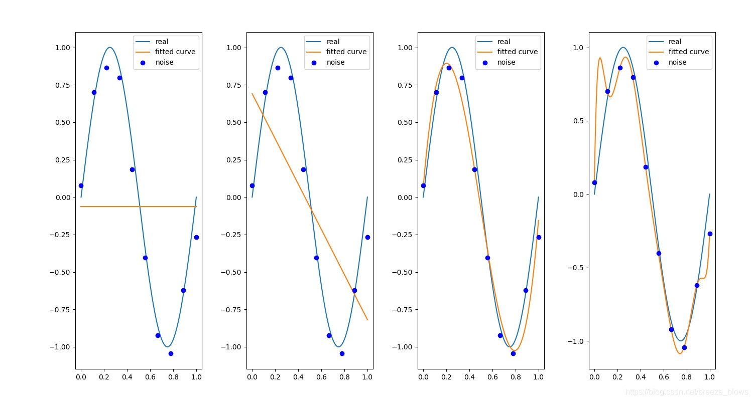
# 十个点'
x = np.linspace(0, 1, 10)
x_points = np.linspace(0, 1, 1000)
# 加上正态分布噪音的目标函数的值
y_ = real_func(x)
y = [np.random.normal(0, 0.1) + y1 for y1 in y_]

index = 0
plt.figure(figsize=(15, 8))

def fitting(M=0):
    """
    M    为 多项式的次数
    """
    # 随机初始化多项式参数
    p_init = np.random.rand(M + 1)
    # 最小二乘法
    p_lsq = leastsq(residuals_func, p_init, args=(x, y))
    #p_lsq = leastsq(residuals_func_regularization, p_init, args=(x, y)) #加入正则化
    print('Fitting Parameters:', p_lsq[0])

    # 可视化
    plt.subplot(141 + index)
    plt.plot(x_points, real_func(x_points), label='real')
    plt.plot(x_points, fit_func(p_lsq[0], x_points), label='fitted curve')
    plt.plot(x, y, 'bo', label='noise')
    plt.legend()
    return p_lsq



for i in [0, 1, 3, 9]:
    lsq_0 = fitting(i)
    index += 1

plt.subplots_adjust(top=0.92, bottom=0.08, left=0.10, right=0.95, hspace=0.25,
                        wspace=0.35) #调整子图间距

plt.savefig("demo.jpg")
plt.show()

正则化前

正则化后

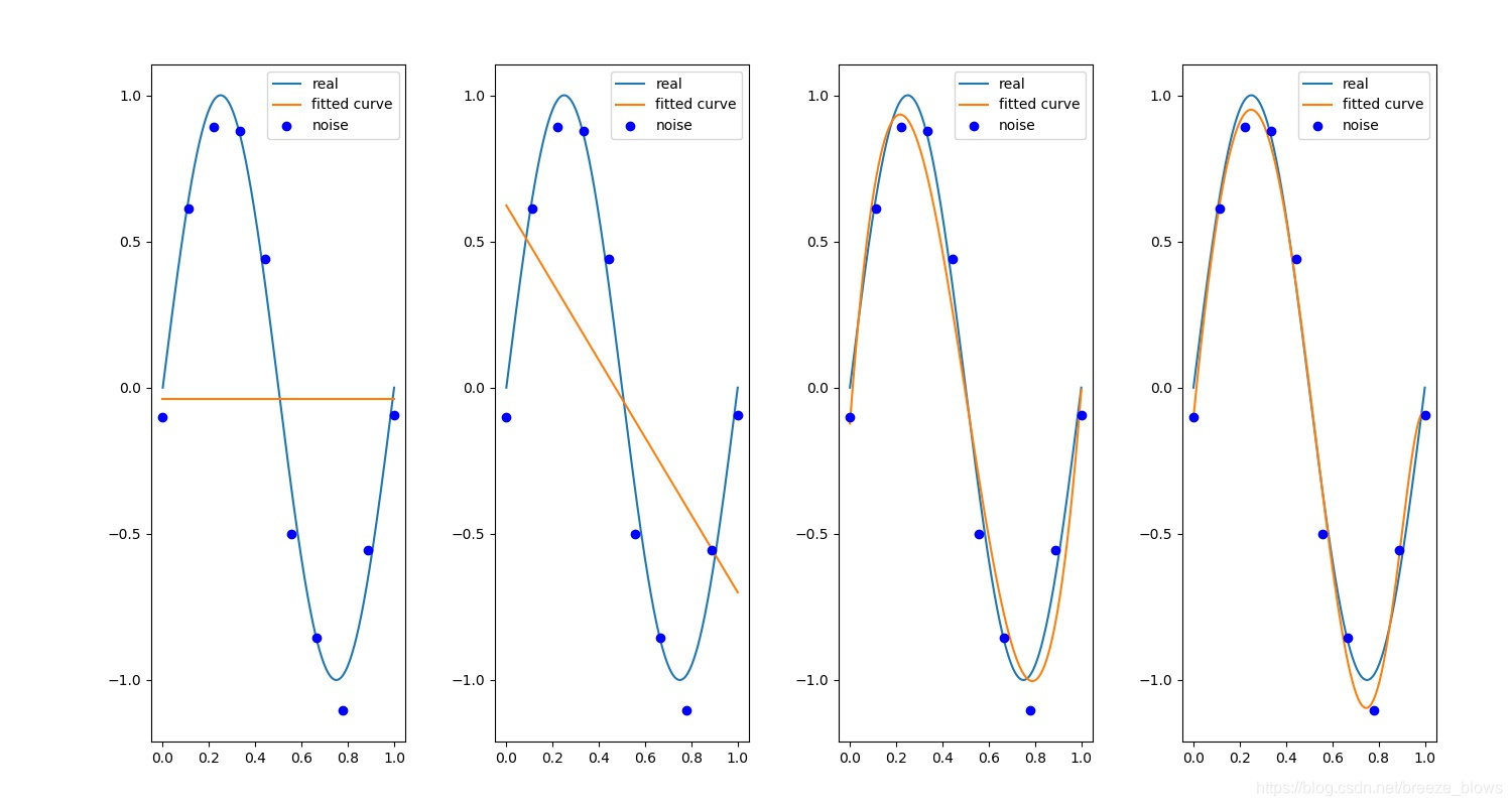
可以明显看出正则化的作用