批标准化（Batch Normalization）、Tensorflow实现Batch Normalization

批标准化（Batch Normalization）：

论文：Batch Normalization: Accelerating Deep Network Training by Reducing Internal Covariate Shift

论文地址：https://arxiv.org/pdf/1502.03167.pdf

Batch Normalization的基本思想：

深层神经网络在每一层做线性变换(y=wx+b)后，得到的值随着网络深度加深或者在训练过程中，其分布会逐渐发生偏移或者变动，之所以训练收敛慢，一般是整体分布逐渐往非线性函数(如sigmoid函数)的取值区间的上下限两端靠近，这会导致反向传播时低层神经网络的梯度消失，这就是训练深层神经网络收敛越来越慢的本质原因。

Batch Normalization就是通过一定的规范化手段，把线性变换后得到的值的分布强行拉回到均值为0方差为1的标准正态分布，这样使得这些值落在非线性函数中对输入比较敏感的区域，这样输入值的小变化就会导致损失函数较大的变化，梯度就会变大，避免梯度消失的问题。而且梯度变大意味着学习收敛速度快，能大大加快训练速度。

Batch Normalization训练神经网络模型的步骤：

首先，求每一个训练批次输入数据的均值：

然后，求每一个训练批次输入数据的方差：

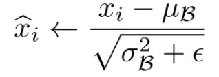
使用求得的均值和方差对该批次的训练数据做归一化，获得0-1分布(其中ε是为了避免除数为0时所使用的微小正数)：

由于归一化后的基本会被限制在正态分布下，这会使得网络的表达能力下降。

为解决该问题，我们引入两个新的参数：γ,β。 γ和β是在训练时网络自己学习得到的，它们用来恢复要学习的特征。

我们将乘以γ调整数值大小，再加上β增加偏移后得到，这里的γ是尺度因子，β是平移因子。

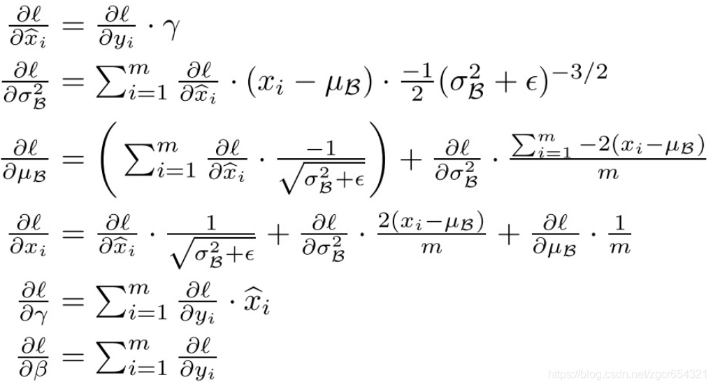
在训练过程中，我们还需要计算反向传播loss函数的梯度，并且计算每个参数（注意：γ 和 β）。我们使用链式法则，如下所示：

Batch Normalization测试神经网络模型的步骤：

测试时我们没有mini-batch，但我们可以用下面几种方法计算出进行归一化时的平均值和方差。

方法1：

即平均值为所有mini-batch的平均值的平均值，而方差为每个batch的方差的无偏估计；

方法2：

使用我们之前介绍过的指数加权平均（exponentially weighted average）的方法来预测测试过程单个样本的和。对于第层隐藏层，考虑所有mini-batch在该隐藏层下的和，然后用指数加权平均的方式来预测得到当前单个样本的和。这样就实现了对测试过程单个样本的均值和方差估计。最后，再利用训练过程得到的γ和 β值计算出各层的值。

举例说明：

为什么我们要把线性变换后的输出值调整成均值为0，方差为1的标准正态分布？

首先看正态分布的图：

由上图我们可知，在一个标准差范围内，也就是x值落在[-1,1]的范围内的概率为68%，在两个标准差范围内，也就是说x值落在[-2,2]的范围内的概率为95%。

我们再看一下sigmoid(x)函数的图像：

现在我们假设没有经过Batch Normalization调整前的x值满足均值是-6、方差是1的正态分布，那么就有95%的值落在了[-8,-4]之间，此时对应的sigmoid(x)的值接近于0，这个区域的导数值很小，函数值变化很慢。而假设经过Batch Normalization调整后的x值满足均值是0、方差是1的正态分布，那么就有95%的x值落在了[-2,2]区间内，这一段区间内sigmoid(x)函数的导数值比较大，函数变化较快，故这个区域的梯度变化也比较大。

因此，经过Batch Normalization调整后，x值落到了梯度变化较大的区间，这样我们训练时权重更新的幅度就比较大，训练过程就会加快。

另外，BN为了保证非线性的获得，对变换后的满足均值为0方差为1的x又进行了scale加上shift操作(y=scale*x+shift)，每个神经元增加了两个参数scale和shift参数，这两个参数是通过训练学习到的，意思是通过scale和shift把这个值从标准正态分布左移或者右移一点并长胖一点或者变瘦一点，每个实例挪动的程度不一样，这样等价于非线性函数的值从正中心周围的线性区往非线性区动了动。

Batch Normalization的优点：

对于深层的神经网络，每一层都使用Batch Normalization就可以使得不同层的权重变化整体步调更一致，这样可以使用更高的学习率，加快训练速度；

Batch Normalization可以防止过拟合。因此如果我们用了Batch Normalization，此时就可以移除或使用较低的dropout，降低L2权重衰减系数等防止过拟合的手段。论文中最后的模型分别使用10%、5%和0%的dropout训练模型，与之前的40%-50%相比，可以大大提高训练速度。

输入的标准化处理Normalizing inputs和隐藏层的标准化处理Batch Normalization是有区别的：

Normalizing inputs使所有输入数据的均值为0，方差为1。而Batch Normalization可使各隐藏层输入的均值和方差为任意值（因为Batch Normalization进行转换后还会进行y=scale*x+shift操作）。

Tensorflow实现Batch Normalization：

代码如下：

import tensorflow as tf
import tqdm
import matplotlib.pyplot as plt
import os
from tensorflow.examples.tutorials.mnist import input_data

os.environ['TF_CPP_MIN_LOG_LEVEL'] = '2'
os.environ["CUDA_VISIBLE_DEVICES"] = '0'
mnist = input_data.read_data_sets("MNIST_data", one_hot=True)

X = tf.placeholder(tf.float32, shape=[None, 784])
Y = tf.placeholder(tf.float32, shape=[None, 10])
# dropout比率
KEEP_PROB = tf.placeholder(tf.float32)
# 是否在训练阶段
IS_TRAINING = tf.placeholder(tf.bool)
USE_BN = tf.placeholder(tf.bool)
iteration = 3000

# 定义4个全连接层的变量，这是一个4层的全连接神经网络
w_1 = tf.Variable(tf.random_normal([784, 300]))
b_1 = tf.Variable(tf.constant(0.1, shape=[300]))
w_2 = tf.Variable(tf.random_normal([300, 100]))
b_2 = tf.Variable(tf.constant(0.1, shape=[100]))
w_3 = tf.Variable(tf.random_normal([100, 100]))
b_3 = tf.Variable(tf.constant(0.1, shape=[100]))
w_4 = tf.Variable(tf.random_normal([100, 10]))
b_4 = tf.Variable(tf.constant(0.1, shape=[10]))
# 定义第1层、第2层、第3层中的BN过程中的beta和gamma变量
gamma_1 = tf.Variable(tf.ones([300]))
beta_1 = tf.Variable(tf.zeros([300]))
gamma_2 = tf.Variable(tf.ones([100]))
beta_2 = tf.Variable(tf.zeros([100]))
gamma_3 = tf.Variable(tf.ones([100]))
beta_3 = tf.Variable(tf.zeros([100]))


# BN函数
def batch_norm(x, gamma, beta, is_training, use_bn, decay=0.99, eps=1e-3):
	# 先判断要不要用BN，再判断目前使用BN是在训练阶段还是测试阶段
	if use_bn is False:
		return x
	# 求一个批样本的平均值和方差
	batch_mean, batch_var = tf.nn.moments(x, [0, 1])
	# tf.train.ExponentialMovingAverage实现滑动平均模型，它使用指数衰减来计算变量的移动平均值。
	# decay是衰减率。在创建ExponentialMovingAverage对象时，需指定衰减率（decay），用于控制模型的更新速度。
	# ExponentialMovingAverage对每一个待更新训练学习的变量/variable都会维护一个影子变量/shadow variable
	# 影子变量的初始值与训练变量的初始值相同。当运行变量更新时，每个影子变量都会更新为：
	# shadow variable=decay∗shadow variable+(1−decay)∗variable
	ema = tf.train.ExponentialMovingAverage(decay=decay)

	def mean_var_with_update():
		# 这里的[batch_mean, batch_var]就是影子变量
		# ema_apply_op = ema.apply([next1,next2,nex3...])，这里传入的[next1,next2,nex3...]是一个变量列表，可以同时计算多个加权平均数
		# total1 = a * total1 + (1 - a) * next1, total2 = a * total2 + (1 - a) * next2
		ema_apply_op = ema.apply([batch_mean, batch_var])
		# tf.control_dependencies()给图中的某些计算指定顺序，与tf.identity配合使用的话，可以达到这样的效果：
		# 先运行ema_apply_op更新了batch_mean, batch_var变量后，用tf.identity(batch_mean)将更新后的batch_mean值取出
		with tf.control_dependencies([ema_apply_op]):
			return tf.identity(batch_mean), tf.identity(batch_var)

	# tf.cond相当于一个三目运算符，如果is_training为True，则取mean_var_with_update的结果，否则取后面lambda的结果
	# 需要注意的是在运行时后面两种结果都被计算出来了，只是我们选择取哪种结果继续下面的运算
	mean, var = tf.cond(is_training, mean_var_with_update, lambda: (ema.average(batch_mean), ema.average(batch_var)))
	# 对x进行批标准化
	normed = tf.nn.batch_normalization(x, mean, var, beta, gamma, eps)
	return normed


# 定义cnn模型
def model(x, y, keep_prob, is_training, use_bn):
	# 定义了一个4层的全连接神经网络
	layer1_out = tf.add(tf.matmul(x, w_1), b_1)
	layer1_out = batch_norm(layer1_out, gamma_1, beta_1, is_training, use_bn)
	layer1_out_activation = tf.nn.relu(layer1_out)
	layer1_out_dropout = tf.nn.dropout(layer1_out_activation, keep_prob)

	layer2_out = tf.add(tf.matmul(layer1_out_dropout, w_2), b_2)
	layer2_out = batch_norm(layer2_out, gamma_2, beta_2, is_training, use_bn)
	layer2_out_activation = tf.nn.relu(layer2_out)
	layer2_out_dropout = tf.nn.dropout(layer2_out_activation, keep_prob)

	layer3_out = tf.add(tf.matmul(layer2_out_dropout, w_3), b_3)
	layer3_out = batch_norm(layer3_out, gamma_3, beta_3, is_training, use_bn)
	layer3_out_activation = tf.nn.relu(layer3_out)
	layer3_out_dropout = tf.nn.dropout(layer3_out_activation, keep_prob)

	layer_out = tf.nn.softmax(tf.add(tf.matmul(layer3_out_dropout, w_4), b_4))

	cost = tf.reduce_mean(-tf.reduce_sum(y * tf.log(layer_out)))
	optimizer = tf.train.AdamOptimizer(learning_rate=0.002).minimize(cost)
	correct_prediction = tf.equal(tf.argmax(y, 1), tf.argmax(layer_out, 1))
	accuracy = tf.reduce_mean(tf.cast(correct_prediction, tf.float32))
	return cost, optimizer, accuracy


loss, op, acc = model(X, Y, KEEP_PROB, IS_TRAINING, USE_BN)

tf.set_random_seed(1)
bn_acc_record = []
bn_acc_step = []
total_average_bn_loss_step = []
total_average_bn_loss = []
# 迭代训练2000次，记录使用了BN时的loss和acc
with tf.Session() as sess_bn:
	sess_bn.run(tf.global_variables_initializer())
	total_bn_loss = 0
	# tqdm包可以将训练过程像进度条一样显示出来,并且可显示已用时间/剩余时间
	for i in tqdm.tqdm(range(iteration)):
		train_batch_x_data, train_batch_y_data = mnist.train.next_batch(64)
		bn_loss, _ = sess_bn.run([loss, op],
								 feed_dict={X: train_batch_x_data, Y: train_batch_y_data, KEEP_PROB: 0.8,
											IS_TRAINING: True, USE_BN: True})
		total_bn_loss += bn_loss
		if i > 100:
			total_average_bn_loss_step.append(i)
			total_average_bn_loss.append(total_bn_loss / (i + 1))
		if i % 50 == 0:
			test_batch_x_data, test_batch_y_data = mnist.test.next_batch(64)
			bn_acc = sess_bn.run([acc],
								 feed_dict={X: test_batch_x_data, Y: test_batch_y_data, KEEP_PROB: 1.0,
											IS_TRAINING: False, USE_BN: True})

			bn_acc_step.append(i)
			bn_acc_record.append(bn_acc[0])

# 为了让两个模型更具有可比性，将其tf变量种子设成一样，这样它们初始化时的值一样
tf.set_random_seed(1)
no_bn_acc_record = []
no_bn_acc_step = []
total_average_no_bn_loss_step = []
total_average_no_bn_loss = []
# 迭代训练2000次，记录不使用BN时的loss和acc
with tf.Session() as sess_no_bn:
	sess_no_bn.run(tf.global_variables_initializer())
	total_no_bn_loss = 0
	for i in tqdm.tqdm(range(iteration)):
		train_batch_x_data, train_batch_y_data = mnist.train.next_batch(64)
		no_bn_loss, _ = sess_no_bn.run([loss, op],
									   feed_dict={X: train_batch_x_data, Y: train_batch_y_data, KEEP_PROB: 0.8,
												  IS_TRAINING: True, USE_BN: False})
		total_no_bn_loss += no_bn_loss
		if i > 100:
			total_average_no_bn_loss_step.append(i)
			total_average_no_bn_loss.append(total_bn_loss / (i + 1))
		if i % 50 == 0:
			test_batch_x_data, test_batch_y_data = mnist.test.next_batch(64)
			no_bn_acc = sess_no_bn.run([acc],
									   feed_dict={X: test_batch_x_data, Y: test_batch_y_data, KEEP_PROB: 1.0,
												  IS_TRAINING: False, USE_BN: False})
			no_bn_acc_step.append(i)
			no_bn_acc_record.append(no_bn_acc[0])

# 将使用和不使用BN时的loss变化和acc变化画成图做对比
fig, ax = plt.subplots(1, 2, figsize=(12, 8))
ax[0].set(title='total average loss')
ax[1].set(title='acc')
ax[0].plot(total_average_bn_loss_step, total_average_bn_loss, '-', color='red', label=r'$bn\_loss$')
ax[0].plot(total_average_no_bn_loss_step, total_average_no_bn_loss, '-', color='blue', label=r'$no\_bn\_loss$')
ax[0].legend(loc="upper right")
ax[1].plot(bn_acc_step, bn_acc_record, '-', color='red', label=r'$bn\_acc$')
ax[1].plot(no_bn_acc_step, no_bn_acc_record, '-', color='blue', label=r'$no\_bn\_loss$')
ax[1].legend(loc="upper right")
plt.show()
plt.close()

这个模型使用mnist为训练数据，模型是一个4层的全连接神经网络，我们在每个神经层使用BN和每个神经层不使用BN各训练3000次，观察这个过程中total average loss的变化和acc的变化。

运行结果如下：

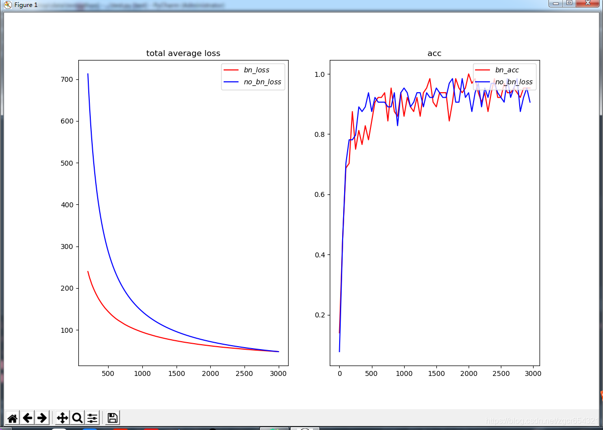
我们可以看到使用了BN后的模型loss值下降的更快，模型训练的速度加快了。