什么是批标准化?
批标准化(Batch Normalization)是深度学习中常用的一种技术,旨在加速神经网络的训练过程并提高模型的收敛速度。
批标准化通过在神经网络的每一层中对输入数据进行标准化来实现。具体而言,对于每个输入样本,在每一层的前向传播过程中,都会计算其均值和方差,并使用批量内的均值和方差对输入进行标准化。标准化后的数据会经过缩放和平移操作,使得网络可以学习到适合当前任务的特定数据分布。这样做的好处包括:
1.收敛速度更快:批标准化有助于避免梯度消失和梯度爆炸问题,使得神经网络在训练过程中更快地收敛。
2.允许更高的学习率:标准化输入可以使学习率的选择更加宽松,使得学习过程更加稳定。
3.正则化作用:批标准化在一定程度上具有正则化的效果,有助于防止过拟合。
4.不那么依赖初始化:由于标准化的存在,对网络的初始权重设置并不像传统网络那样敏感,这简化了网络的初始化过程。
对比使用批标准化和不使用批标准化
import torch
from torch import nn
from torch.nn import init
import torch.utils.data as Data
import matplotlib.pyplot as plt
import numpy as np
# 用于可复现
# torch.manual_seed(1) # reproducible
# np.random.seed(1)
# Hyper parameters
# 样本点
N_SAMPLES = 2000
# 批大小
BATCH_SIZE = 64
# 轮次
EPOCH = 12
# 学习率
LR = 0.03
# 隐藏层层数
N_HIDDEN = 8
# 激活函数
ACTIVATION = torch.tanh
B_INIT = -0.2 # use a bad bias constant initializer
# training data
# 生成-7到10之间的N_SAMPLES个值的等差数列,并将其转化为一个二维列向量
x = np.linspace(-7, 10, N_SAMPLES)[:, np.newaxis]
# 生成一个均值为0,标准差为2的和x相同形状的噪声数据
noise = np.random.normal(0, 2, x.shape)
# 生成x对应的y值
y = np.square(x) - 5 + noise
# test data
test_x = np.linspace(-7, 10, 200)[:, np.newaxis]
noise = np.random.normal(0, 2, test_x.shape)
test_y = np.square(test_x) - 5 + noise
train_x = torch.from_numpy(x).float()
train_y = torch.from_numpy(y).float()
test_x = torch.from_numpy(test_x).float()
test_y = torch.from_numpy(test_y).float()
train_dataset = Data.TensorDataset(train_x, train_y)
train_loader = Data.DataLoader(dataset=train_dataset, batch_size=BATCH_SIZE, shuffle=True, num_workers=2,)
# show data
# plt.scatter(train_x.numpy(), train_y.numpy(), c='#FF9359', s=50, alpha=0.2, label='train')
# plt.scatter(test_x.numpy(), test_y.numpy(), c='blue', s=50, alpha=0.2, label='test')
# plt.legend(loc='best')
class Net(nn.Module):
def __init__(self, batch_normalization=False):
super(Net, self).__init__()
# 是否进行批标准化
self.do_bn = batch_normalization
# 全连接层的列表
self.fcs = []
# 批标准化层的列表
self.bns = []
self.bn_input = nn.BatchNorm1d(1, momentum=0.5) # for input data
for i in range(N_HIDDEN): # build hidden layers and BN layers
# 如果是第一层,输入神经元个数为1,其余为10个
input_size = 1 if i == 0 else 10
# 全连接层
fc = nn.Linear(input_size, 10)
# 将全连接层重新命名然后设置为类属性
setattr(self, 'fc%i' % i, fc) # IMPORTANT set layer to the Module
# 对全连接层的参数进行初始化
self._set_init(fc) # parameters initialization
# 添加到列表中
self.fcs.append(fc)
if self.do_bn:
bn = nn.BatchNorm1d(10, momentum=0.5)
setattr(self, 'bn%i' % i, bn) # IMPORTANT set layer to the Module
self.bns.append(bn)
self.predict = nn.Linear(10, 1) # output layer
self._set_init(self.predict) # parameters initialization
def _set_init(self, layer):
init.normal_(layer.weight, mean=0., std=.1)
init.constant_(layer.bias, B_INIT)
# 前向传播
def forward(self, x):
pre_activation = [x]
if self.do_bn:
x = self.bn_input(x) # input batch normalization
layer_input = [x]
for i in range(N_HIDDEN):
x = self.fcs[i](x)
pre_activation.append(x)
if self.do_bn: x = self.bns[i](x) # batch normalization
x = ACTIVATION(x)
layer_input.append(x)
out = self.predict(x)
# 返回预测值、每个隐藏层的输入、激活函数的输出
return out, layer_input, pre_activation
nets = [Net(batch_normalization=False), Net(batch_normalization=True)]
# print(*nets) # print net architecture
# 优化器
opts = [torch.optim.Adam(net.parameters(), lr=LR) for net in nets]
# MSE作为损失函数
loss_func = torch.nn.MSELoss()
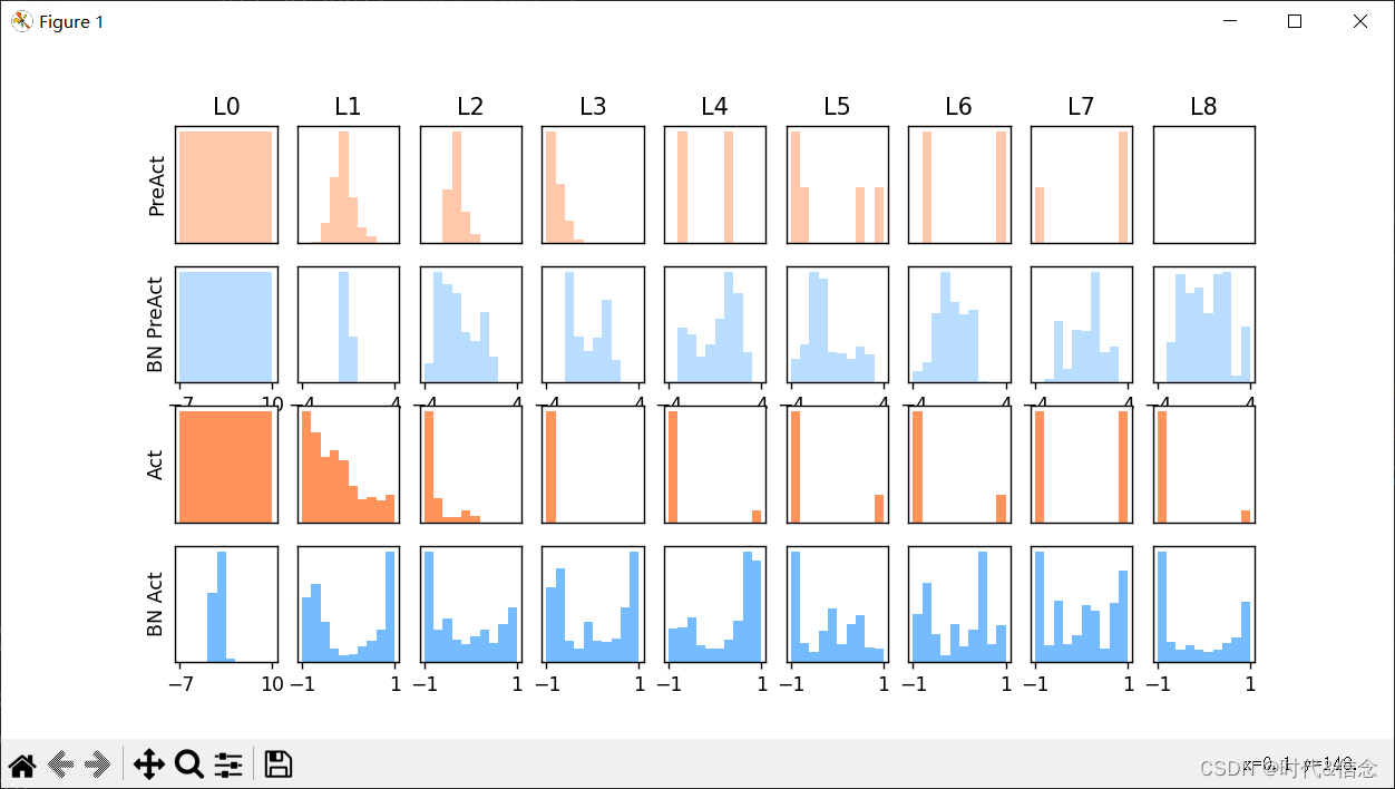
def plot_histogram(l_in, l_in_bn, pre_ac, pre_ac_bn):
for i, (ax_pa, ax_pa_bn, ax, ax_bn) in enumerate(zip(axs[0, :], axs[1, :], axs[2, :], axs[3, :])):
[a.clear() for a in [ax_pa, ax_pa_bn, ax, ax_bn]]
if i == 0:
p_range = (-7, 10);the_range = (-7, 10)
else:
p_range = (-4, 4);the_range = (-1, 1)
ax_pa.set_title('L' + str(i))
ax_pa.hist(pre_ac[i].data.numpy().ravel(), bins=10, range=p_range, color='#FF9359', alpha=0.5);ax_pa_bn.hist(pre_ac_bn[i].data.numpy().ravel(), bins=10, range=p_range, color='#74BCFF', alpha=0.5)
ax.hist(l_in[i].data.numpy().ravel(), bins=10, range=the_range, color='#FF9359');ax_bn.hist(l_in_bn[i].data.numpy().ravel(), bins=10, range=the_range, color='#74BCFF')
for a in [ax_pa, ax, ax_pa_bn, ax_bn]: a.set_yticks(());a.set_xticks(())
ax_pa_bn.set_xticks(p_range);ax_bn.set_xticks(the_range)
axs[0, 0].set_ylabel('PreAct');axs[1, 0].set_ylabel('BN PreAct');axs[2, 0].set_ylabel('Act');axs[3, 0].set_ylabel('BN Act')
plt.pause(0.01)
if __name__ == "__main__":
f, axs = plt.subplots(4, N_HIDDEN + 1, figsize=(10, 5))
# 开启动态绘制
plt.ion() # something about plotting
plt.show()
# training
losses = [[], []] # recode loss for two networks
for epoch in range(EPOCH):
print('Epoch: ', epoch)
layer_inputs, pre_acts = [], []
# 训练两个网络
for net, l in zip(nets, losses):
net.eval() # set eval mode to fix moving_mean and moving_var
pred, layer_input, pre_act = net(test_x)
l.append(loss_func(pred, test_y).data.item())
layer_inputs.append(layer_input)
pre_acts.append(pre_act)
net.train() # free moving_mean and moving_var
plot_histogram(*layer_inputs, *pre_acts) # plot histogram
for step, (b_x, b_y) in enumerate(train_loader):
for net, opt in zip(nets, opts): # train for each network
# 获取到预测值
pred, _, _ = net(b_x)
# 计算loss
loss = loss_func(pred, b_y)
# 梯度清零
opt.zero_grad()
# 误差反向传播
loss.backward()
# 逐步优化网络参数
opt.step() # it will also learns the parameters in Batch Normalization
# 关闭动态绘制
plt.ioff()
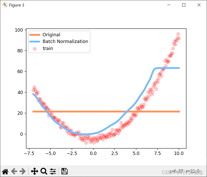
# plot training loss
# 绘制loss图
plt.figure(2)
plt.plot(losses[0], c='#FF9359', lw=3, label='Original')
plt.plot(losses[1], c='#74BCFF', lw=3, label='Batch Normalization')
plt.xlabel('step')
plt.ylabel('test loss')
plt.ylim((0, 2000))
plt.legend(loc='best')
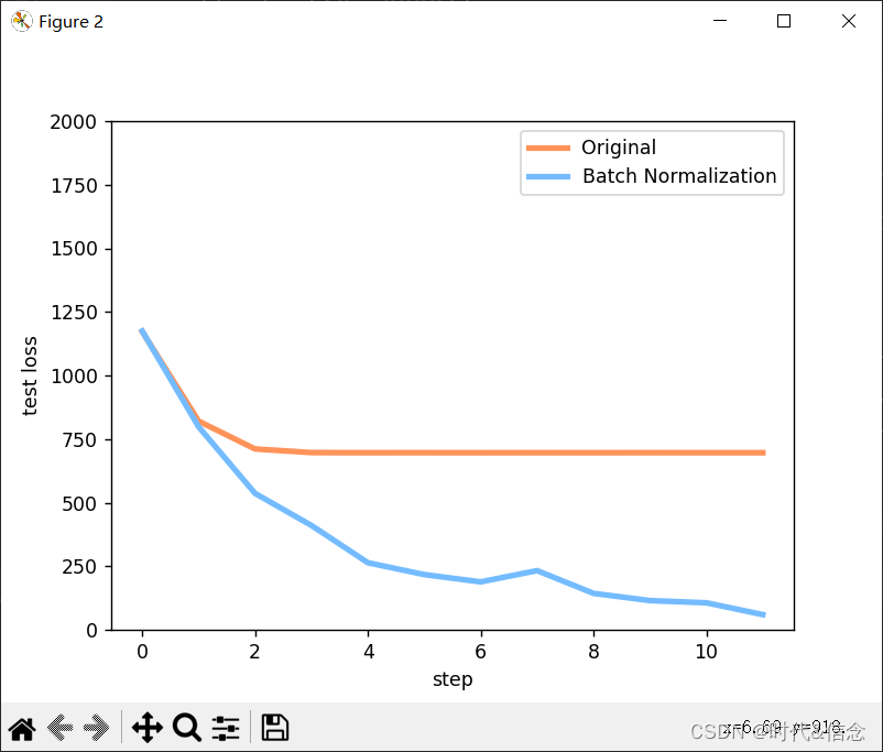
# evaluation
# set net to eval mode to freeze the parameters in batch normalization layers
[net.eval() for net in nets] # set eval mode to fix moving_mean and moving_var
preds = [net(test_x)[0] for net in nets]
plt.figure(3)
# 测试拟合效果
plt.plot(test_x.data.numpy(), preds[0].data.numpy(), c='#FF9359', lw=4, label='Original')
plt.plot(test_x.data.numpy(), preds[1].data.numpy(), c='#74BCFF', lw=4, label='Batch Normalization')
plt.scatter(test_x.data.numpy(), test_y.data.numpy(), c='r', s=50, alpha=0.2, label='train')
plt.legend(loc='best')
plt.show()
运行结果